PyTorch nn.CrossEntropyLoss() 交叉熵损失函数详解和要点提醒
文章目录
- 前置知识
- nn.CrossEntropyLoss() 交叉熵损失
- 参数
- 数学公式
- 带权重的公式(weight)
- 标签平滑(label_smoothing)
- 要点
- 附录
- 参考链接
前置知识
深度学习:关于损失函数的一些前置知识(PyTorch Loss)
nn.CrossEntropyLoss() 交叉熵损失
torch.nn.CrossEntropyLoss(weight=None, size_average=None, ignore_index=-100, reduce=None, reduction='mean', label_smoothing=0.0)This criterion computes the cross entropy loss between input logits and target.
该函数计算输入 logits 和目标之间的交叉熵损失。
参数
- weight (Tensor, 可选): 一个形状为 ( C ) (C) (C) 的张量,表示每个类别的权重。如果提供了这个参数,损失函数会根据类别的权重来调整各类别的损失,适用于类别不平衡的问题。默认值是
None。 - size_average (bool, 可选): 已弃用。如果
reduction不是'none',则默认情况下损失是取平均(True);否则,是求和(False)。默认值是None。 - ignore_index (int, 可选): 如果指定了这个参数,则该类别的索引会被忽略,不会对损失和梯度产生影响。默认值是
-100。 - reduce (bool, 可选): 已弃用。请使用
reduction参数。默认值是None。 - reduction (str, 可选): 指定应用于输出的归约方式。可选值为
'none'、'mean'、'sum'。'none'表示不进行归约,'mean'表示对所有样本的损失求平均,'sum'表示对所有样本的损失求和。默认值是'mean'。 - label_smoothing (float, 可选): 标签平滑值,范围在 [0.0, 1.0] 之间。默认值是
0.0。标签平滑是一种正则化技术,通过在真实标签上添加一定程度的平滑来避免过拟合。
数学公式
附录部分会验证下述公式和代码的一致性。
假设有 N N N 个样本,每个样本属于 C C C 个类别之一。对于第 i i i 个样本,它的真实类别标签为 y i y_i yi,模型的输出 logits 为 x i = ( x i 1 , x i 2 , … , x i C ) \mathbf{x}_i = (x_{i1}, x_{i2}, \ldots, x_{iC}) xi=(xi1,xi2,…,xiC),其中 x i c x_{ic} xic 表示第 i i i 个样本在第 c c c 类别上的原始输出分数(logits)。
交叉熵损失的计算步骤如下:
- Softmax 函数:
对 logits 进行 softmax 操作,将其转换为概率分布:
p i c = exp ( x i c ) ∑ j = 1 C exp ( x i j ) p_{ic} = \frac{\exp(x_{ic})}{\sum_{j=1}^{C} \exp(x_{ij})} pic=∑j=1Cexp(xij)exp(xic)
其中 $ p_{ic} $ 表示第 $ i $ 个样本属于第 $ c $ 类别的预测概率。 - 负对数似然(Negative Log-Likelihood):
计算负对数似然:
ℓ i = − log ( p i y i ) \ell_i = -\log(p_{iy_i}) ℓi=−log(piyi)
其中 ℓ i \ell_i ℓi 是第 i i i 个样本的损失, p i y i p_{iy_i} piyi 表示第 i i i 个样本在真实类别 y i y_i yi 上的预测概率。 - 总损失:
计算所有样本的平均损失(reduction参数默认为'mean'):
L = 1 N ∑ i = 1 N ℓ i = 1 N ∑ i = 1 N − log ( p i y i ) \mathcal{L} = \frac{1}{N} \sum_{i=1}^{N} \ell_i = \frac{1}{N} \sum_{i=1}^{N} -\log(p_{iy_i}) L=N1i=1∑Nℓi=N1i=1∑N−log(piyi)
如果reduction参数为'sum',总损失为所有样本损失的和:
L = ∑ i = 1 N ℓ i = ∑ i = 1 N − log ( p i y i ) \mathcal{L} = \sum_{i=1}^{N} \ell_i = \sum_{i=1}^{N} -\log(p_{iy_i}) L=i=1∑Nℓi=i=1∑N−log(piyi)
如果reduction参数为'none',则返回每个样本的损失 ℓ i \ell_i ℓi 组成的张量。
L = [ ℓ 1 , ℓ 2 , … , ℓ N ] = [ − log ( p i y 1 ) , − log ( p i y 2 ) , … , − log ( p i y N ) ] \mathcal{L} = [\ell_1, \ell_2, \ldots, \ell_N] = [-\log(p_{iy_1}), -\log(p_{iy_2}), \ldots, -\log(p_{iy_N})] L=[ℓ1,ℓ2,…,ℓN]=[−log(piy1),−log(piy2),…,−log(piyN)]
带权重的公式(weight)
如果指定了类别权重 w = ( w 1 , w 2 , … , w C ) \mathbf{w} = (w_1, w_2, \ldots, w_C) w=(w1,w2,…,wC),则总损失公式为:
L = 1 N ∑ i = 1 N w y i ⋅ ℓ i = ∑ i = 1 N w y i ⋅ ( − log ( p i y i ) ) ∑ i = 1 N w y i \mathcal{L} = \frac{1}{N} \sum_{i=1}^{N} w_{y_i} \cdot \ell_i = \frac{\sum_{i=1}^{N} w_{y_i} \cdot (-\log(p_{iy_i}))}{\sum_{i=1}^{N} w_{y_i}} L=N1i=1∑Nwyi⋅ℓi=∑i=1Nwyi∑i=1Nwyi⋅(−log(piyi))
其中 w y i w_{y_i} wyi 是第 i i i 个样本真实类别的权重。
标签平滑(label_smoothing)
如果标签平滑(label smoothing)参数 α \alpha α 被启用,目标标签 y i \mathbf{y}_i yi 会被平滑处理:
y i ′ = ( 1 − α ) ⋅ y i + α C \mathbf{y}_i' = (1 - \alpha) \cdot \mathbf{y}_i + \frac{\alpha}{C} yi′=(1−α)⋅yi+Cα
其中, y i \mathbf{y}_i yi 是原始的 one-hot 编码目标标签, y i ′ \mathbf{y}_i' yi′ 是平滑后的标签。
总的损失公式会相应调整:
ℓ i = − ∑ c = 1 C y i c ′ ⋅ log ( p i c ) \ell_i = - \sum_{c=1}^{C} y_{ic}' \cdot \log(p_{ic}) ℓi=−c=1∑Cyic′⋅log(pic)
其中, y i c y_{ic} yic 是第 i i i 个样本在第 c c c 类别上的标签,为原标签 y i y_i yi 经过 one-hot 编码后 y i \mathbf{y}_i yi 中的值。对于一个 one-hot 编码标签向量, y i c y_{ic} yic 在样本属于类别 c c c 时为 1,否则为 0。
要点
nn.CrossEntropyLoss()接受的输入是 logits,这说明分类的输出不需要提前经过 softmax。如果提前经过 softmax,则需要使用nn.NLLLoss()(负对数似然损失)。import torch import torch.nn as nn import torch.nn.functional as F# 定义输入和目标标签 logits = torch.tensor([[2.0, 0.5], [0.5, 2.0]]) # 未经过 softmax 的 logits target = torch.tensor([0, 1]) # 目标标签# 使用 nn.CrossEntropyLoss 计算损失(接受 logits) criterion_ce = nn.CrossEntropyLoss() loss_ce = criterion_ce(logits, target)# 使用 softmax 后再使用 nn.NLLLoss 计算损失 log_probs = F.log_softmax(logits, dim=1) criterion_nll = nn.NLLLoss() loss_nll = criterion_nll(log_probs, target)print(f"Loss using nn.CrossEntropyLoss: {loss_ce.item()}") print(f"Loss using softmax + nn.NLLLoss: {loss_nll.item()}")# 验证两者是否相等 assert torch.allclose(loss_ce, loss_nll), "The losses are not equal, which indicates a mistake in the assumption." print("The losses are equal, indicating that nn.CrossEntropyLoss internally applies softmax.")
拓展: F.log_softmax()>>> Loss using nn.CrossEntropyLoss: 0.2014133334159851 >>> Loss using softmax + nn.NLLLoss: 0.2014133334159851 >>> The losses are equal, indicating that nn.CrossEntropyLoss internally applies softmax.
F.log_softmax等价于先应用softmax激活函数,然后对结果取对数 log()。它是将softmax和log这两个操作结合在一起,以提高数值稳定性和计算效率。具体的数学定义如下:
log_softmax ( x i ) = log ( softmax ( x i ) ) = log ( exp ( x i ) ∑ j exp ( x j ) ) = x i − log ( ∑ j exp ( x j ) ) \text{log\_softmax}(x_i) = \log\left(\text{softmax}(x_i)\right) = \log\left(\frac{\exp(x_i)}{\sum_j \exp(x_j)}\right) = x_i - \log\left(\sum_j \exp(x_j)\right) log_softmax(xi)=log(softmax(xi))=log(∑jexp(xj)exp(xi))=xi−log(j∑exp(xj))
在代码中,F.log_softmax的等价操作可以用以下步骤实现:- 计算
softmax。 - 计算
softmax的结果的对数。
import torch
import torch.nn.functional as F# 定义输入 logits
logits = torch.tensor([[2.0, 1.0, 0.1], [1.0, 3.0, 0.2]])# 计算 log_softmax
log_softmax_result = F.log_softmax(logits, dim=1)# 分开计算 softmax 和 log
softmax_result = F.softmax(logits, dim=1)
log_result = torch.log(softmax_result)print("Logits:")
print(logits)print("\nLog softmax (using F.log_softmax):")
print(log_softmax_result)print("\nSoftmax result:")
print(softmax_result)print("\nLog of softmax result:")
print(log_result)# 验证两者是否相等
assert torch.allclose(log_softmax_result, log_result), "The results are not equal."
print("\nThe results are equal, indicating that F.log_softmax is equivalent to softmax followed by log.")
从结果中可以看到>>> Logits: >>> tensor([[2.0000, 1.0000, 0.1000], >>> [1.0000, 3.0000, 0.2000]])>>> Log softmax (using F.log_softmax): >>> tensor([[-0.4170, -1.4170, -2.3170], >>> [-2.1791, -0.1791, -2.9791]])>>> Softmax result: >>> tensor([[0.6590, 0.2424, 0.0986], >>> [0.1131, 0.8360, 0.0508]])>>> Log of softmax result: >>> tensor([[-0.4170, -1.4170, -2.3170], >>> [-2.1791, -0.1791, -2.9791]])>>> The results are equal, indicating that F.log_softmax is equivalent to softmax followed by log.F.log_softmax的结果等价于先计算 softmax 再取对数。- 计算
nn.CrossEntropyLoss()实际上默认(reduction=‘mean’)计算的是每个样本的平均损失,已经做了归一化处理,所以不需要对得到的结果进一步除以 batch_size 或其他某个数,除非是用作 loss_weight。下面是一个简单的例子:import torch import torch.nn as nn# 定义损失函数 criterion = nn.CrossEntropyLoss()# 定义输入和目标标签 input1 = torch.tensor([[2.0, 0.5], [0.5, 2.0]], requires_grad=True) # 批量大小为 2 target1 = torch.tensor([0, 1]) # 对应的目标标签input2 = torch.tensor([[2.0, 0.5], [0.5, 2.0], [2.0, 0.5], [0.5, 2.0]], requires_grad=True) # 批量大小为 4 target2 = torch.tensor([0, 1, 0, 1]) # 对应的目标标签# 计算损失 loss1 = criterion(input1, target1) loss2 = criterion(input2, target2)print(f"Loss with batch size 2: {loss1.item()}") print(f"Loss with batch size 4: {loss2.item()}")
可以看到这里的>>> Loss with batch size 2: 0.2014133334159851 >>> Loss with batch size 4: 0.2014133334159851input2实际上等价于torch.cat([input1, input1], dim=0),target2等价于torch.cat([target1, target1], dim=0),简单拓展了 batch_size 大小但最终的 Loss 没变,这也就验证了之前的说法。- 目标标签
target期望两种格式:-
类别索引: 类别的整数索引,而不是 one-hot 编码。范围在 [ 0 , C ) [0, C) [0,C) 之间,其中 C C C 是类别数。如果指定了
ignore_index,则该类别索引也会被接受(即便可能不在类别范围内)
使用示例:# Example of target with class indices import torch import torch.nn as nnloss = nn.CrossEntropyLoss() input = torch.randn(3, 5, requires_grad=True) target = torch.empty(3, dtype=torch.long).random_(5) output = loss(input, target) output.backward() -
类别概率: 类别的概率分布,适用于需要每个批次项有多个类别标签的情况,如标签平滑等。
使用示例:# Example of target with class probabilities import torch import torch.nn as nnloss = nn.CrossEntropyLoss() input = torch.randn(3, 5, requires_grad=True) target = torch.randn(3, 5).softmax(dim=1) output = loss(input, target) output.backward()The performance of this criterion is generally better when target contains class indices, as this allows for optimized computation. Consider providing target as class probabilities only when a single class label per minibatch item is too restrictive.
通常情况下,当目标为类别索引时,该函数的性能更好,因为这样可以进行优化计算。只有在每个批次项的单一类别标签过于限制时,才考虑使用类别概率。
-
附录
用于验证数学公式和函数实际运行的一致性
import torch
import torch.nn.functional as F# 假设有两个样本,每个样本有三个类别
logits = torch.tensor([[1.5, 2.0, 0.5], [1.0, 0.5, 2.5]], requires_grad=True)
targets = torch.tensor([1, 2])# 根据公式实现 softmax
def softmax(x):return torch.exp(x) / torch.exp(x).sum(dim=1, keepdim=True)# 根据公式实现 log-softmax
def log_softmax(x):return x - torch.log(torch.exp(x).sum(dim=1, keepdim=True))# 根据公式实现负对数似然损失(NLLLoss)
def nll_loss(log_probs, targets):N = log_probs.size(0)return -log_probs[range(N), targets].mean()# 根据公式实现交叉熵损失
def custom_cross_entropy(logits, targets):log_probs = log_softmax(logits)return nll_loss(log_probs, targets)# 使用 PyTorch 计算交叉熵损失
criterion = torch.nn.CrossEntropyLoss(reduction='mean')
loss_torch = criterion(logits, targets)# 使用根据公式实现的交叉熵损失
loss_custom = custom_cross_entropy(logits, targets)# 打印结果
print("PyTorch 计算的交叉熵损失:", loss_torch.item())
print("根据公式实现的交叉熵损失:", loss_custom.item())# 验证结果是否相等
assert torch.isclose(loss_torch, loss_custom), "数学公式验证失败"# 带权重的交叉熵损失
weights = torch.tensor([0.7, 0.2, 0.1])
criterion_weighted = torch.nn.CrossEntropyLoss(weight=weights, reduction='mean')
loss_weighted_torch = criterion_weighted(logits, targets)# 根据公式实现带权重的交叉熵损失
def custom_weighted_cross_entropy(logits, targets, weights):log_probs = log_softmax(logits)N = logits.size(0)weighted_loss = -log_probs[range(N), targets] * weights[targets]return weighted_loss.sum() / weights[targets].sum()loss_weighted_custom = custom_weighted_cross_entropy(logits, targets, weights)# 打印结果
print("PyTorch 计算的带权重的交叉熵损失:", loss_weighted_torch.item())
print("根据公式实现的带权重的交叉熵损失:", loss_weighted_custom.item())# 验证结果是否相等
assert torch.isclose(loss_weighted_torch, loss_weighted_custom, atol=1e-6), "带权重的数学公式验证失败"# 标签平滑的交叉熵损失
alpha = 0.1
criterion_label_smoothing = torch.nn.CrossEntropyLoss(label_smoothing=alpha, reduction='mean')
loss_label_smoothing_torch = criterion_label_smoothing(logits, targets)# 根据公式实现标签平滑的交叉熵损失
def custom_label_smoothing_cross_entropy(logits, targets, alpha):N, C = logits.size()log_probs = log_softmax(logits)one_hot = torch.zeros_like(log_probs).scatter(1, targets.view(-1, 1), 1)smooth_targets = (1 - alpha) * one_hot + alpha / Closs = - (smooth_targets * log_probs).sum(dim=1).mean()return lossloss_label_smoothing_custom = custom_label_smoothing_cross_entropy(logits, targets, alpha)# 打印结果
print("PyTorch 计算的标签平滑的交叉熵损失:", loss_label_smoothing_torch.item())
print("根据公式实现的标签平滑的交叉熵损失:", loss_label_smoothing_custom.item())# 验证结果是否相等
assert torch.isclose(loss_label_smoothing_torch, loss_label_smoothing_custom, atol=1e-6), "标签平滑的数学公式验证失败"
>>> PyTorch 计算的交叉熵损失: 0.45524317026138306
>>> 根据公式实现的交叉熵损失: 0.4552431106567383
>>> PyTorch 计算的带权重的交叉熵损失: 0.5048722624778748
>>> 根据公式实现的带权重的交叉熵损失: 0.50487220287323
>>> PyTorch 计算的标签平滑的交叉熵损失: 0.5469098091125488
>>> 根据公式实现的标签平滑的交叉熵损失: 0.5469098091125488
输出没有抛出 AssertionError,验证通过。
参考链接
CrossEntropyLoss - Docs
相关文章:
 交叉熵损失函数详解和要点提醒)
PyTorch nn.CrossEntropyLoss() 交叉熵损失函数详解和要点提醒
文章目录 前置知识nn.CrossEntropyLoss() 交叉熵损失参数数学公式带权重的公式(weight)标签平滑(label_smoothing) 要点 附录参考链接 前置知识 深度学习:关于损失函数的一些前置知识(PyTorch Loss&#x…...

DW学习笔记|数学建模task2
本章主要涉及到的知识点有: 微分方程的解法如何用 Python 解微分方程偏微分方程及其求解方法微分方程的基本案例差分方程的求解数值计算方法元胞自动机 2.1 微分方程的理论基础 微分方程是什么?如果你参加过高考,可能在高三备考中遇到过这…...
【大数据 复习】第9章 数据仓库分析工具Hive
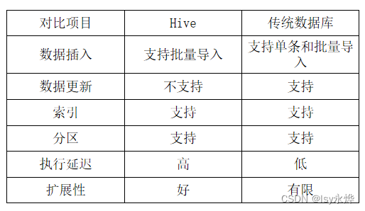
一、概念 1.概述 (1)Hive是一个构建于Hadoop顶层的数据仓库工具。 (2)某种程度上可以看作是用户编程接口,本身不存储和处理数据。 (3)依赖分布式文件系统HDFS存储数据。 (4…...

ionic7 从安装 到 项目启动最后打包成 apk
报错处理 在打包的时候遇到过几个问题,这里记录下来两个 Visual Studio Code运行ionic build出错显示ionic : 无法加载文件 ionic 项目通过 android studio 打开报错 capacitor.settings.gradle 文件不存在 说明 由于之前使用的是 ionic 3,当时打包的…...
setInterval 定时任务执行时间不准验证
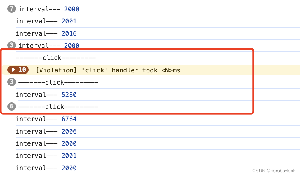
一般在处理定时任务的时候都使用setInterval间隔定时调用任务。 setInterval(() > {console.log("interval"); }, 2 * 1000);我们定义的是两秒执行一次,但是浏览器实际执行的间隔时间只多不少。这是由于浏览器执行 JS 是单线程模式,使用se…...

Stable Diffusion Model网站
Civitai Models | Discover Free Stable Diffusion Modelshttps://www.tjsky.net/tutorial/488https://zhuanlan.zhihu.com/p/610298913超详细的 Stable Diffusion ComfyUI 基础教程(一):安装与常用插件 - 优设网 - 学设计上优设 (uisdc.com)…...
K8S - 实现statefulset 有状态service的灰度发布
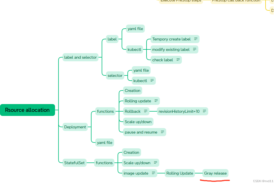
什么是灰度发布 Canary Release 参考 理解 什么是 滚动更新,蓝绿部署,灰度发布 以及它们的区别 配置partition in updateStrategy/rollingUpdate 这次我为修改了 statefulset 的1个yaml file statefulsets/stateful-nginx-without-pvc.yaml: --- apiVe…...

Qt 技术博客:深入理解 Qt 中的 delete 和 deleteLater 与信号槽机制
在 Qt 开发中,内存管理和对象生命周期的处理是至关重要的一环。特别是在涉及信号和槽机制时,如何正确删除对象会直接影响应用程序的稳定性。本文将详细讨论在使用 Qt 的信号和槽机制时,delete 和 deleteLater 的工作原理,并给出最…...

自学鸿蒙HarmonyOS的ArkTS语言<一>基本语法
一、一个ArkTs的目录结构 二、一个页面的结构 A、装饰器 Entry 装饰器 : 标记组件为入口组件,一个页面由多个自定义组件组成,但是只能有一个组件被标记 Component : 自定义组件, 仅能装饰struct关键字声明的数据结构 State:组件中的状态变量…...
)】)
【OpenGauss源码学习 —— (ALTER TABLE(列存修改列类型))】
ALTER TABLE(列存修改列类型) ATExecAlterColumnType 函数1. 检查和处理列存储表的字符集:2. 处理自动递增列的数据类型检查:3. 处理生成列的类型转换检查:4. 处理生成列的数据类型转换: build_column_defa…...
【大数据 复习】第7章 MapReduce(重中之重)
一、概念 1.MapReduce 设计就是“计算向数据靠拢”,而不是“数据向计算靠拢”,因为移动,数据需要大量的网络传输开销。 2.Hadoop MapReduce是分布式并行编程模型MapReduce的开源实现。 3.特点 (1)非共享式,…...

Zookeeper:节点
文章目录 一、节点类型二、监听器及节点删除三、创建节点四、监听节点变化五、判断节点是否存在 一、节点类型 持久(Persistent):客户端和服务器端断开连接后,创建的节点不删除。 持久化目录节点:客户端与Zookeeper断…...

生产级别的 vue
生产级别的 vue 拆分组件的标识更好的组织你的目录如何解决 props-base 设计的问题transparent component (透明组件)可减缓上述问题provide 和 inject vue-meta 在路由中的使用如何确保用户导航到某个路由自己都重新渲染?测试最佳实践如何制…...
spring-kafka(1)集成方法)
kafka(五)spring-kafka(1)集成方法
一、集成 1、pom依赖 <!--kafka--><dependency><groupId>org.apache.kafka</groupId><artifactId>kafka-clients</artifactId></dependency><dependency><groupId>org.springframework.kafka</groupId><artif…...

Java中的设计模式深度解析
Java中的设计模式深度解析 大家好,我是免费搭建查券返利机器人省钱赚佣金就用微赚淘客系统3.0的小编,也是冬天不穿秋裤,天冷也要风度的程序猿! 在软件开发领域,设计模式是一种被广泛应用的经验总结和解决方案&#x…...

鸿蒙 HarmonyOS NEXT星河版APP应用开发—上篇
一、鸿蒙开发环境搭建 DevEco Studio安装 下载 访问官网:https://developer.huawei.com/consumer/cn/deveco-studio/选择操作系统版本后并注册登录华为账号既可下载安装包 安装 建议:软件和依赖安装目录不要使用中文字符软件安装包下载完成后࿰…...
[FreeRTOS 基础知识] 互斥访问与回环队列 概念
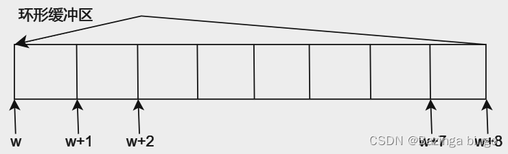
文章目录 为什么需要互斥访问?使用队列实现互斥访问休眠和唤醒机制环形缓冲区 为什么需要互斥访问? 在裸机中,假设有两个函数(func_A, func_B)都要修改a的值(a),那么将a定义为全局变…...
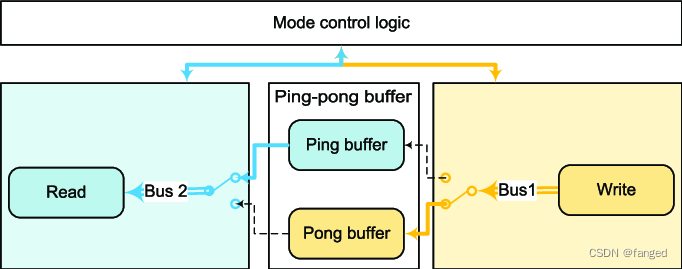
音视频的Buffer处理
最近在做安卓下UVC的一个案子。正好之前搞过ST方案的开机广告,这个也是我少数最后没搞成功的项目。当时也有点客观原因,当时ST要退出机顶盒市场,所以一切的支持都停了,当时啃他家播放器几十万行的代码,而且几乎没有文档…...

【总结】攻击 AI 模型的方法
数据投毒 污染训练数据 后门攻击 通过设计隐蔽的触发器,使得模型在正常测试时无异常,而面对触发器样本时被操纵输出。后门攻击可以看作是特殊的数据投毒,但是也可以通过修改模型参数来实现 对抗样本 只对输入做微小的改动,使模型…...
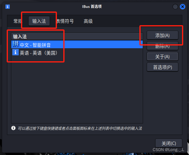
Linux配置中文环境
文章目录 前言中文语言包中文输入法中文字体 前言 在Linux系统中修改为中文环境,通常涉及以下几个步骤: 中文语言包 更新源列表: 更新系统的软件源列表和语言环境设置,确保可以安装所需的语言包。 sudo apt update sudo apt ins…...

Linux内核PCIe热插拔驱动开发实战:从IDT芯片到稳定运行
1. 项目概述与核心价值最近在搞一个嵌入式设备项目,需要实现PCIe设备的热插拔支持。这玩意儿在服务器、存储阵列和工业控制领域太常见了,但真要在Linux内核里把它做稳定、做可靠,里面的门道可不少。我这次折腾的,就是一个基于Linu…...
)
Elasticsearch 7.6.1 实战:从零构建招聘信息搜索服务(索引、数据与分页)
1. 从零搭建招聘搜索服务:为什么选择Elasticsearch? 最近在帮朋友改造招聘网站的后台搜索功能时,我果断推荐了Elasticsearch 7.6.1。这个版本在稳定性和功能完整性上达到了很好的平衡,特别适合中小型企业的搜索场景。相比传统数据…...
)
【免费下载】 AD7124中文手册(非常完整)
AD7124中文手册(非常完整) 【下载地址】AD7124中文手册非常完整 AD7124-8是一款高性能模拟前端,设计用于在各种苛刻环境中实现精确的数据采集。这款芯片的特点在于其内置的高精度24位Σ-Δ模数转换器(ADC),能够灵活配置以支持8个差…...

换背景照片怎么制作?一篇全网最全的AI抠图工具对比指南
最近经常有朋友问我:"怎样才能快速换背景照片啊?"确实,随着自媒体时代的到来,无论是做电商展示产品、准备证件照,还是制作社交媒体内容,都离不开换背景这个需求。今天我就把这两年用过的所有抠图…...
)
TVA智能体范式的工业视觉革命(8)
重磅预告:本专栏将独家连载系列丛书《智能体视觉技术与应用》部分精华内容,该书是世界首套系统阐述“因式智能体”视觉理论与实践的专著,特邀美国 TypeOne 公司首席科学家、斯坦福大学博士 Bohan 担任技术顾问。Bohan先生师从美国三院院士、“…...
:从图灵机到 ECU)
从沙子到车辙(1.5):从图灵机到 ECU
1.5 从图灵机到 ECU 一座恶魔般的机房 1945 年,费城,宾夕法尼亚大学摩尔工程学院。 一座 30 吨重的巨兽蹲在一间约 167 平方米的机房里。它的名字叫 ENIAC(Electronic Numerical Integrator and Computer)——世界上第一台通用…...

从Typora迁移到Obsidian,我踩过的那些坑和高效配置方案
从Typora迁移到Obsidian:无缝过渡的深度实践指南 当我在2022年决定将积累了5年的技术笔记库从Typora迁移到Obsidian时,最初以为只是换个编辑器那么简单。直到实际操作时才发现,这两个看似相似的Markdown工具在使用哲学和操作细节上存在诸多差…...

[2026降本增效实战] 制造业生产成本核算如何提升准确性?基于实在Agent的端到端解决方案
在2026年的工业4.0深水区,制造业的竞争早已从单纯的产能比拼转向了极致的成本精度博弈。 传统的成本核算模式正面临前所未有的挑战:数据颗粒度过粗、跨系统断点频发、人工干预导致的误差难以溯源。 随着大模型技术与超自动化技术的深度融合,智…...

永强数据恢复硬盘设备加密数据专业解锁恢复服务
在当今数字化时代,数据的重要性不言而喻。无论是个人用户存储的珍贵照片、视频,还是企业存储的关键商业数据,一旦丢失,都可能带来巨大的损失。而硬盘设备加密数据的丢失或无法解锁,更是让人头疼不已。北京永强数据恢复…...

避开安全门调试大坑:详解西门子SFDOOR指令的3个关键参数与常见故障复位
西门子SFDOOR指令实战排错手册:3个关键参数解析与故障复位技巧 1. 安全门控制的核心逻辑与典型故障模式 在工业自动化现场,安全门作为保护人员安全的关键设备,其可靠性直接关系到生产系统的稳定运行。西门子SFDOOR功能块通过双通道信号检测和…...