第三份代码:VoxelNet的pytorch实现
VoxelNet是点云体素化处理的最开始的网络结构设计,通过完全弄明白整个VoxelNet的pytorch实现是非常有必要的。
参考的代码是这一份:GitHub - RPFey/voxelnet_pytorch: modification of voxelnet
参考文章:VoxelNet论文解读和代码解析_voxel-rcnn论文和逐代码解析-CSDN博客
数据集下载百度云:https://pan.baidu.com/s/19qfeWI6GLPB_esgQjezOsw
密码:hsg5
(一)crop.py文件
数据预处理:先使用crop.py程序把图像坐标之外的点云剪裁掉便于后期可视化验证,在运行crop.py之前,需要先在training和testing文件夹下新建crop文件夹,运行完的数据存在里面。
# 这个文件只需要调用系统库:作为一个预处理函数的存在
import numpy as np
import cv2
import sys# 我记得CAM是其中的一模块,这里暂且将其作为一个模块计数变量
CAM = 2
#----------这个函数从filename中读取所有的激光雷达传感器数据,并且转换为numpy:nx4大小形状
# 取一个包含点云数据的二进制文件,每个点由四个浮点数表示(通常是 x、y、z 坐标和强度)。
# 函数返回一个 NumPy 数组,其中包含了这些点的数据。
# 这种格式的数据通常来自于 Velodyne 激光雷达传感器。
def load_velodyne_points(filename):points = np.fromfile(filename, dtype=np.float32).reshape(-1, 4)#points = points[:, :3]  # exclude luminancereturn points# calib_dir这个文件名起的,老吓人了 —— 哦哦! camera calibration相机标定--先不管了
def load_calib(calib_dir):# P2 * R0_rect * Tr_velo_to_cam * ylines = open(calib_dir).readlines()lines = [ line.split()[1:] for line in lines ][:-1] # 每一行作为[]list中的一个元素,除了第一行# 这个CAM=2的变量就用到这里了将第lines[CAM]的元素reshape为[3,4]的形状P = np.array(lines[CAM]).reshape(3,4)# 同样的将lines[5]进行reshape  - -这个将作为刚体变换Tr_velo_to_cam = np.array(lines[5]).reshape(3,4)  # 下面还有将它concate为4x4的numpy matrixTr_velo_to_cam = np.concatenate( [ Tr_velo_to_cam, np.array([0,0,0,1]).reshape(1,4) ] , 0 )# np.eye生成的就是单位矩阵 - -这个将作为旋转矩阵R_cam_to_rect = np.eye(4)R_cam_to_rect[:3,:3] = np.array(lines[4][:9]).reshape(3,3)# 这三个矩阵的元素都设置为float32类型的,然后返回这三个矩阵作为后续的使用,这里的函数只是生成这3个矩阵P = P.astype('float32')Tr_velo_to_cam = Tr_velo_to_cam.astype('float32')R_cam_to_rect = R_cam_to_rect.astype('float32')return P, Tr_velo_to_cam, R_cam_to_rect# prepare提前预处理 Velodyne 激光雷达的数据信息 -- 函数1
# 选出反射率大于 0 的点,将它们的反射率统一设置为 1,并转置点云数据,使其适合用于相机投影矩阵的计算。
def prepare_velo_points(pts3d_raw):'''Replaces the reflectance value by 1, and tranposes the array, sopoints can be directly multiplied by the camera projection matrix'''pts3d = pts3d_raw# Reflectance > 0indices = pts3d[:, 3] > 0pts3d = pts3d[indices ,:]pts3d[:,3] = 1return pts3d.transpose(), indices# 将3D pc映射到 2D img 中
# 这个函数的作用是将三维点云数据中位于相机前方的点投影到二维图像平面上,并返回这些点的二维图像坐标以及对应的原始三维点。
def project_velo_points_in_img(pts3d, T_cam_velo, Rrect, Prect):'''Project 3D points into 2D image. Expects pts3d as a 4xNnumpy array. Returns the 2D projection of the points thatare in front of the camera only an the corresponding 3D points.'''# 3D points in camera reference frame.# 使用激光雷达到相机的转换矩阵 T_cam_velo 和相机的内参矩阵 Rrect 将三维点云从激光雷达坐标系转换到相机坐标系。pts3d_cam = Rrect.dot(T_cam_velo.dot(pts3d))  # pts3d就是雷达坐标系坐标 list# Before projecting, keep only points with z>0# (points that are in fronto of the camera).# 筛选出相机坐标系下 z 坐标大于0的点,这些点位于相机前方。idx = (pts3d_cam[2,:]>=0)# 使用相机内参矩阵 Prect 将这些三维点投影到二维图像平面上pts2d_cam = Prect.dot(pts3d_cam[:,idx])# 通过将二维坐标的 x 和 y 值除以 z 值来归一化二维图像坐标,得到最终的二维投影点# ------------------------------------------------# 返回位于相机前方的三维点、对应的二维投影点,以及这些点的索引。return pts3d[:, idx], pts2d_cam/pts2d_cam[2,:], idx# 图像数据与对应的三维点云数据对齐,为每个点添加了颜色信息,从而创建了一个丰富的数据集
def align_img_and_pc(img_dir, pc_dir, calib_dir):# 读入img、pts、calibrationimg = cv2.imread(img_dir)pts = load_velodyne_points( pc_dir )P, Tr_velo_to_cam, R_cam_to_rect = load_calib(calib_dir)# 对pts选出反射率大于 0 的点,将它们的反射率统一设置为 1,并转置点云数据,使其适合用于相机投影矩阵的计算。pts3d, indices = prepare_velo_points(pts)pts3d_ori = pts3d.copy()# 返回的indices对应的 反射率强度reflectances = pts[indices, 3]# 将三维点云数据中位于相机前方的点投影到二维图像平面上,并返回这些点的二维图像坐标以及对应的原始三维点。pts3d, pts2d_normed, idx = project_velo_points_in_img( pts3d, Tr_velo_to_cam, R_cam_to_rect, P  )#print reflectances.shape, idx.shapereflectances = reflectances[idx]#print reflectances.shape, pts3d.shape, pts2d_normed.shapeassert reflectances.shape[0] == pts3d.shape[1] == pts2d_normed.shape[1]# rows, cols = img.shape[:2]points = []for i in range(pts2d_normed.shape[1]):c = int(np.round(pts2d_normed[0,i]))r = int(np.round(pts2d_normed[1,i]))if c < cols and r < rows and r > 0 and c > 0:color = img[r, c, :]# 这里的point是配置好所有的属性的pointspoint = [ pts3d[0,i], pts3d[1,i], pts3d[2,i], reflectances[i], color[0], color[1], color[2], pts2d_normed[0,i], pts2d_normed[1,i]  ]points.append(point)points = np.array(points)return points# update the following directories
IMG_ROOT = '/data/cxg1/VoxelNet_pro/Data/training/image_2/'
PC_ROOT = '/data/cxg1/VoxelNet_pro/Data/training/velodyne/'
CALIB_ROOT = '/data/cxg1/VoxelNet_pro/Data/training/calib/'
PC_CROP_ROOT = '/data/cxg1/VoxelNet_pro/Data/training/crop/'  # 这个文件夹暂时没有 -- 输出地址# 这个是当前文件的测试代码:--对7481个对象进行测试
for frame in range(0, 7481):# 依次获取每个对象的文件地址img_dir = IMG_ROOT + '%06d.png' % framepc_dir = PC_ROOT + '%06d.bin' % framecalib_dir = CALIB_ROOT + '%06d.txt' % frame# 调用 align_img_and_pc函数进行 对齐处理 - # 图像数据与对应的三维点云数据对齐,为每个点添加了颜色信息,从而创建了一个丰富的数据集points = align_img_and_pc(img_dir, pc_dir, calib_dir)# 最后的处理 到 输出的地址 -- 还是存储为二进制的格式的文件,之后取出文件都是从这个二进制文件入手的output_name = PC_CROP_ROOT + '%06d.bin' % framesys.stdout.write('Save to %s \n' % output_name)points[:,:4].astype('float32').tofile(output_name)
这里面确实是对原始的kitti数据集里面的数据进行预处理,并且把预处理后的数据存储到了crop文件夹中,之后kitti dataset其实是从这个crop文件中构建的
(二)kitti.py文件
这个文件,虽然主要是构建一个KittiDataset。但里面的核心操作是,如何进行Voxelize体素化的操作。
from __future__ import division
import os
import os.path
import torch.utils.data as data
import utils
from utils import box3d_corner_to_center_batch, anchors_center_to_corner, corner_to_standup_box2d_batch
from data_aug import aug_data
from box_overlaps import bbox_overlaps
import numpy as np
import cv2
import torch
from detectron2.layers.rotated_boxes import pairwise_iou_rotated# 它的代码里面处理Kitti_Dataset还是值得借鉴的
class KittiDataset(data.Dataset):def __init__(self, cfg, root='./KITTI',set='train',type='velodyne_train'):# 设置好模块变量self.type = typeself.root = rootself.data_path = os.path.join(root, 'training')self.lidar_path = os.path.join(self.data_path, "crop")      # 这里获取的lidar数据是crop处理之后self.image_path = os.path.join(self.data_path, "image_2/")self.calib_path = os.path.join(self.data_path, "calib")self.label_path = os.path.join(self.data_path, "label_2")# 打开对应的txt文件with open(os.path.join(self.data_path, '%s.txt' % set)) as f:self.file_list = f.read().splitlines()# cfg配置变量的设置self.T = cfg.Tself.vd = cfg.vdself.vh = cfg.vhself.vw = cfg.vwself.xrange = cfg.xrangeself.yrange = cfg.yrangeself.zrange = cfg.zrangeself.anchors = torch.tensor(cfg.anchors.reshape(-1,7)).float().to(cfg.device)self.anchors_xylwr = self.anchors[..., [0, 1, 5, 4, 6]].contiguous()self.feature_map_shape = (int(cfg.H / 2), int(cfg.W / 2))self.anchors_per_position = cfg.anchors_per_positionself.pos_threshold = cfg.pos_thresholdself.neg_threshold = cfg.neg_thresholddef cal_target(self, gt_box3d, gt_xyzhwlr, cfg):# Input:#   labels: (N,)#   feature_map_shape: (w, l)#   anchors: (w, l, 2, 7)# Output:#   pos_equal_one (w, l, 2)#   neg_equal_one (w, l, 2)#   targets (w, l, 14)# attention: cal IoU on birdviewanchors_d = torch.sqrt(self.anchors[:, 4] ** 2 + self.anchors[:, 5] ** 2).to(cfg.device)# denote whether the anchor box is pos or negpos_equal_one = torch.zeros((*self.feature_map_shape, 2)).to(cfg.device)neg_equal_one = torch.zeros((*self.feature_map_shape, 2)).to(cfg.device)targets = torch.zeros((*self.feature_map_shape, 14)).to(cfg.device)gt_xyzhwlr = torch.tensor(gt_xyzhwlr, requires_grad=False).float().to(cfg.device)gt_xylwr = gt_xyzhwlr[..., [0, 1, 5, 4, 6]]# BOTTLENECKiou = pairwise_iou_rotated(self.anchors_xylwr,gt_xylwr.contiguous()).cpu().numpy() # (gt - anchor)id_highest = np.argmax(iou.T, axis=1)  # the maximum anchor's IDid_highest_gt = np.arange(iou.T.shape[0])mask = iou.T[id_highest_gt, id_highest] > 0 # make sure all the iou is positiveid_highest, id_highest_gt = id_highest[mask], id_highest_gt[mask]# find anchor iou > cfg.XXX_POS_IOUid_pos, id_pos_gt = np.where(iou > self.pos_threshold)# find anchor iou < cfg.XXX_NEG_IOUid_neg = np.where(np.sum(iou < self.neg_threshold,axis=1) == iou.shape[1])[0] # anchor doesn't match ant ground truthfor gt in range(iou.shape[1]):if gt not in id_pos_gt and iou[id_highest[gt], gt] > self.neg_threshold:id_pos = np.append(id_pos, id_highest[gt])id_pos_gt = np.append(id_pos_gt, gt)# sample the negative points to keep ratio as 1:10 with minimum 500num_neg = 10 * id_pos.shape[0]if num_neg < 500:num_neg = 500if id_neg.shape[0] > num_neg:np.random.shuffle(id_neg)id_neg = id_neg[:num_neg]# cal the target and set the equal oneindex_x, index_y, index_z = np.unravel_index(id_pos, (*self.feature_map_shape, self.anchors_per_position))pos_equal_one[index_x, index_y, index_z] = 1# ATTENTION: index_z should be np.array# parameterize the ground truth box relative to anchor boxstargets[index_x, index_y, np.array(index_z) * 7] = \(gt_xyzhwlr[id_pos_gt, 0] - self.anchors[id_pos, 0]) / anchors_d[id_pos]targets[index_x, index_y, np.array(index_z) * 7 + 1] = \(gt_xyzhwlr[id_pos_gt, 1] - self.anchors[id_pos, 1]) / anchors_d[id_pos]targets[index_x, index_y, np.array(index_z) * 7 + 2] = \(gt_xyzhwlr[id_pos_gt, 2] - self.anchors[id_pos, 2]) / self.anchors[id_pos, 3]targets[index_x, index_y, np.array(index_z) * 7 + 3] = torch.log(gt_xyzhwlr[id_pos_gt, 3] / self.anchors[id_pos, 3])targets[index_x, index_y, np.array(index_z) * 7 + 4] = torch.log(gt_xyzhwlr[id_pos_gt, 4] / self.anchors[id_pos, 4])targets[index_x, index_y, np.array(index_z) * 7 + 5] = torch.log(gt_xyzhwlr[id_pos_gt, 5] / self.anchors[id_pos, 5])targets[index_x, index_y, np.array(index_z) * 7 + 6] = (gt_xyzhwlr[id_pos_gt, 6] - self.anchors[id_pos, 6])index_x, index_y, index_z = np.unravel_index(id_neg, (*self.feature_map_shape, self.anchors_per_position))neg_equal_one[index_x, index_y, index_z] = 1return pos_equal_one, neg_equal_one, targetsdef preprocess(self, lidar):# This func cluster the points in the same voxel.# shuffling the pointsnp.random.shuffle(lidar)voxel_coords = ((lidar[:, :3] - np.array([self.xrange[0], self.yrange[0], self.zrange[0]])) / (self.vw, self.vh, self.vd)).astype(np.int32)# convert to  (D, H, W)voxel_coords = voxel_coords[:,[2,1,0]]#具体来说,np.unique 函数的返回值如下:#voxel_coords:包含输入数组中所有唯一体素坐标的数组。#inv_ind:一个与输入数组 voxel_coords 形状相同的数组,其中的每个元素是指向 voxel_coords 中对应唯一值的索引。#这意味着 voxel_coords[inv_ind] 将与原始的 voxel_coords 数组相同。#voxel_counts:一个数组,其中的每个元素表示对应唯一体素坐标在原始 voxel_coords 数组中出现的次数。voxel_coords, inv_ind, voxel_counts = np.unique(voxel_coords, axis=0, \return_inverse=True, return_counts=True)# 其实上面几行代码基本就是完成了voxelize体素化,下面不过是循环对 每个voxel体素进行处理voxel_features = []# 总共len个体素for i in range(len(voxel_coords)):voxel = np.zeros((self.T, 7), dtype=np.float32)# 选出所有处于体素i的pointpts = lidar[inv_ind == i]# 值取前self.T的pointif voxel_counts[i] > self.T:pts = pts[:self.T, :]voxel_counts[i] = self.T# augment the points# voxel_features就是一个存储每个 voxel的list,每个元素就是这个voxel,然后正好可以和voxel_coords对应起来# 原始的点云数据和中心化后的坐标拼接在一起,形成一个新的特征数组。voxel[:pts.shape[0], :] = np.concatenate((pts, pts[:, :3] - np.mean(pts[:, :3], 0)), axis=1)voxel_features.append(voxel)# 返回voxel_features的array以及对应的coords原体素坐标轴return np.array(voxel_features), voxel_coords# 算了,我觉得dataset这个模块的设计关键是看 __getitem__(self,i)怎么设计的def __getitem__(self, i):# 获取对应的路径变量lidar_file = self.lidar_path + '/' + self.file_list[i] + '.bin'calib_file = self.calib_path + '/' + self.file_list[i] + '.txt'label_file = self.label_path + '/' + self.file_list[i] + '.txt'image_file = self.image_path + '/' + self.file_list[i] + '.png'# 重点是获取label中修正后的ground_truth_box3d的位置 、 以及对应的ladar数据的输入# 其实,就是相当于 input 和 label数据calib = utils.load_kitti_calib(calib_file)Tr = calib['Tr_velo2cam']gt_box3d_corner, gt_box3d = utils.load_kitti_label(label_file, Tr)lidar = np.fromfile(lidar_file, dtype=np.float32).reshape(-1, 4)# 区分 train 和 test两种不同的返回处理if self.type == 'velodyne_train':image = cv2.imread(image_file)# data augmentation# lidar, gt_box3d = aug_data(lidar, gt_box3d)# specify a range# 进一步处理输入和输出lidar, gt_box3d_corner, gt_box3d = utils.get_filtered_lidar(lidar, gt_box3d_corner, gt_box3d)# voxelize# 通过调用self.preprocess对输入的lidar数据进行voxelizevoxel_features, voxel_coords = self.preprocess(lidar)# bounding-box encoding# pos_equal_one, neg_equal_one, targets = self.cal_target(gt_box3d_corner, gt_box3d)# 返回的是 体素化后的features和坐标coords  、 以及对应的 ground_truth label数据 、 以及image 、其他return voxel_features, voxel_coords, gt_box3d_corner, gt_box3d, image, calib, self.file_list[i] # pos_equal_one, neg_equal_one, targets, image, calib, self.file_list[i]# 对于test测试的数据的处理更加简洁一些elif self.type == 'velodyne_test':image = cv2.imread(image_file)lidar, gt_box3d = utils.get_filtered_lidar(lidar, gt_box3d)voxel_features, voxel_coords = self.preprocess(lidar)# 返回的结果里面就不包含ground_truth label了return voxel_features, voxel_coords, image, calib, self.file_list[i]else:raise ValueError('the type invalid')def __len__(self):return len(self.file_list)# 这个文件中最重要的就是看明白 里面的preprocess处理 体素的函数操作了!!!!!!!!!!
(三)config.py文件
configure大多数时候,就是放一些全局参数什么的。这里的config.py里面放置最重要的东西就是grid棋盘格,也就是用来规划所有的体素的。
import math
import numpy as np# 其实,config可以理解为其他文件需要用到的 “超参数”
class config:# classesclass_list = ['Car', 'Van']# batch sizeN=2# maxiumum number of points per voxelT=35# voxel sizevd = 0.4vh = 0.2vw = 0.2# points cloud rangexrange = (0.0, 70.4)yrange = (-40, 40)zrange = (-3, 1)# voxel grid -- 这里其实是计算的grid中的voxel的个数W = math.ceil((xrange[1] - xrange[0]) / vw)H = math.ceil((yrange[1] - yrange[0]) / vh)D = math.ceil((zrange[1] - zrange[0]) / vd)# # iou threshold# pos_threshold = 0.9# neg_threshold = 0.45# 点是一组预定义的边界框,用于在目标检测任务中初始化边界框的位置和尺寸# anchors: (200, 176, 2, 7) x y z h w l r# 在x坐标范围内,每隔一个体素宽度生成一个点,直到范围的末端,生成的点数是 W//2。# 在y坐标范围内,每隔一个体素高度生成一个点,直到范围的末端,生成的点数是 H//2。# 虽然不知道为什么是W//2而不是W,????不明白,反正就是生成了grid。欸,不过下面有一个np.tile的操作#x = np.linspace(xrange[0]+vw, xrange[1]-vw, W//2) y = np.linspace(yrange[0]+vh, yrange[1]-vh, H//2)cx, cy = np.meshgrid(x, y)# all is (w, l, 2) # 返回一个形状为 (W//2, H//2, 2) 的新数组# cx = np.tile(cx[..., np.newaxis], 2) cy = np.tile(cy[..., np.newaxis], 2)# # 终于明白那7个参数分别是什么了: x,y,z位置,w,l,h 对应box的长宽高 以及旋转度rcz = np.ones_like(cx) * -1.0  # w = np.ones_like(cx) * 1.6l = np.ones_like(cx) * 3.9h = np.ones_like(cx) * 1.56r = np.ones_like(cx)# anchors就是锚定,anchors的参数就在这里理解# r[..., 0] = 0r[..., 1] = np.pi/2anchors = np.stack([cx, cy, cz, h, w, l, r], axis=-1)anchors_per_position = 2  # non-maximum suppression -- threshold的设置,cuda的个数nms_threshold = 1e-3score_threshold = 0.9#device = "cuda:2"device = "cuda:1"num_dim = 51last_epoch=0
(四)voxelnet.py文件
里面通过 SVFE、Convolution、RPN搭建了网络,重点是RPN的设计 以及 VFE 对体素提特征:
import torch.nn as nn
import torch.nn.functional as F
import torch
from torch.autograd import Variable
from config import config as cfg# 还是以这个RPFey的实现为主,因为这个哥的实现nms算法是用的detectron2的库而不是C++的扩展,nice
# 算了,那个utils.py里面处理kitti的label数据的函数有点小多,先看看这个network# 其实应该是作者的习惯,把Conv2d后面接上batchnorm和relu
# conv2d + bn + relu
class Conv2d(nn.Module):def __init__(self,in_channels,out_channels,k,s,p, activation=True, batch_norm=True):super(Conv2d, self).__init__()self.conv = nn.Conv2d(in_channels,out_channels,kernel_size=k,stride=s,padding=p)if batch_norm:self.bn = nn.BatchNorm2d(out_channels)else:self.bn = Noneself.activation = activationdef forward(self,x):x = self.conv(x)if self.bn is not None:x=self.bn(x)if self.activation:return F.relu(x,inplace=True)else:return x# 果然还是要用到3D卷积,不过其中的原理和2D卷积没有区别
# conv3d + bn + relu
class Conv3d(nn.Module):def __init__(self, in_channels, out_channels, k, s, p, batch_norm=True):super(Conv3d, self).__init__()self.conv = nn.Conv3d(in_channels, out_channels, kernel_size=k, stride=s, padding=p)if batch_norm:self.bn = nn.BatchNorm3d(out_channels)else:self.bn = Nonedef forward(self, x):x = self.conv(x)if self.bn is not None:x = self.bn(x)return F.relu(x, inplace=True)# 估计也是linear + batchnorm + relu
# Fully Connected Network
class FCN(nn.Module):def __init__(self,cin,cout):super(FCN, self).__init__()self.cout = coutself.linear = nn.Linear(cin, cout)self.bn = nn.BatchNorm1d(cout)def forward(self,x):# KK is the stacked k across batchkk, t, _ = x.shapex = self.linear(x.view(kk*t,-1))x = F.relu(self.bn(x))return x.view(kk,t,-1)# Feature encoding ?
# Voxel Feature Encoding layer
class VFE(nn.Module):def __init__(self,cin,cout):super(VFE, self).__init__()assert cout % 2 == 0# 模块变量units和fcnself.units = cout // 2self.fcn = FCN(cin,self.units)def forward(self, x, mask): # 以确定哪些体素(voxels)包含点云数据中的点,哪些是空的# point-wise feauture# 输入的x其实是Nx7的一个array: 而且VFE的输入参数cin和cout,其实应该cin就是输入时的特征维度7,输出cout就是转换后的特征维度#pwf = self.fcn(x) # 此时的pwf已经是NxTxunits的形状了# 局部增强汇聚操作# locally aggregated feature# torch.max(pwf, 1)[0] 返回了一个张量,包含了 pwf 张量沿着维度 1 的最大值。# 这个操作通常用于特征聚合,例如在体素化点云数据时,通过取每个体素内点的最大特征值来表示该体素的特征。# 经过unsqueeze(1)后,从N变成了Nx1的tensor,# 再经过repeat(1.cfg.T,1)的操作后,沿着维度1重复cfg.T次,变成了NxTxunits的维度#laf = torch.max(pwf,1)[0].unsqueeze(1).repeat(1,cfg.T,1)# 哦,point-wise feature其实就是字面意思,是每个点上的feature,比如开始feature的维度是7# point-wise concat feature# 通过cat在dim=2合并之后,本来2个分别是NxTx units和NxTx units,cat之后NxTx 2*units#pwcf = torch.cat((pwf,laf),dim=2)# apply mask# 首先还是要把mask进行变形 -- 至于mask怎么来的,直接去看下面的SVFE结构# 这里输入的mask通过unsqueeze(2)之后,是NxTx1的元素是bool值的# 首先,units*2 == cout,#mask = mask.unsqueeze(2).repeat(1, 1, self.units * 2)# 然后才是用pwcf和mask作点乘# mask也是一个bool的类型,所以在只有非空的体素的feature是不为0的!#pwcf = pwcf * mask.float()return pwcf# Stacked Voxel Feature Encoding
class SVFE(nn.Module):def __init__(self):super(SVFE, self).__init__()# 结构很清楚了,2个VFE 加上 1个FCNself.vfe_1 = VFE(7,32)           # 另外,需要弄明白的是这个VFE的2个参数的含义self.vfe_2 = VFE(32,128)self.fcn = FCN(128,128)def forward(self, x):# mask不是原始输入,而是从这里计算得到的# 利用not equal函数创建一个掩码,该掩码标识输入张量 x 中具有非零最大特征值的点。# maskmask = torch.ne(torch.max(x,2)[0], 0) # 滤掉为零的点# 输入的x其实就是numpy array的voxel_featuresx = self.vfe_1(x, mask)x = self.vfe_2(x, mask)# 算了,这个mask虽然我感觉应该要,不对,mask这么做的合理的,因为mask已经指示了空的地方x = self.fcn(x)  # 此时的x是 NxTx128# element-wise max pooling# 所以返回的就是Nx128x = torch.max(x,1)[0]return x# Convolutional Middle Layer -- 就是3个3D卷积操作
class CML(nn.Module):def __init__(self):super(CML, self).__init__()self.conv3d_1 = Conv3d(128, 64, 3, s=(2, 1, 1), p=(1, 1, 1))self.conv3d_2 = Conv3d(64, 64, 3, s=(1, 1, 1), p=(0, 1, 1))self.conv3d_3 = Conv3d(64, 64, 3, s=(2, 1, 1), p=(1, 1, 1))def forward(self, x):x = self.conv3d_1(x)x = self.conv3d_2(x)x = self.conv3d_3(x)return x# Region Proposal Network —— 这个是重点分析理解的模块实现
# 需要进行mask定位,一般都是需要Region Proposal的
# RPN输出的其实是 前景/背景 分数 + 原图中的坐标位置
class RPN(nn.Module):def __init__(self):super(RPN, self).__init__()# 第一个卷积将H-W --> H/2 W/2  : 也就是一次下采样self.block_1 = [Conv2d(128, 128, 3, 2, 1)]self.block_1 += [Conv2d(128, 128, 3, 1, 1) for _ in range(3)]self.block_1 = nn.Sequential(*self.block_1)# 第二个下采用模块 : 同样是H\W减半self.block_2 = [Conv2d(128, 128, 3, 2, 1)]self.block_2 += [Conv2d(128, 128, 3, 1, 1) for _ in range(5)]self.block_2 = nn.Sequential(*self.block_2)# 第三个下采用模块 : 同样是H\W减半self.block_3 = [Conv2d(128, 256, 3, 2, 1)]self.block_3 += [nn.Conv2d(256, 256, 3, 1, 1) for _ in range(5)]self.block_3 = nn.Sequential(*self.block_3)# 上采样模块up sampling: 分别增大H和W的4倍 、 2倍 和 1倍self.deconv_1 = nn.Sequential(nn.ConvTranspose2d(256, 256, 4, 4, 0),nn.BatchNorm2d(256))self.deconv_2 = nn.Sequential(nn.ConvTranspose2d(128, 256, 2, 2, 0),nn.BatchNorm2d(256))self.deconv_3 = nn.Sequential(nn.ConvTranspose2d(128, 256, 1, 1, 0),nn.BatchNorm2d(256))# 两个head都是简单的Con2d的设计# anchors_per_position就是2个anchors,cfg参数就是2# socre只要每个位置有 前景/背景 两个分数即可。 而reg需要的是每个位置有 7个参数?????# 7个参数:x,y,z位置+l,w,h,r长宽高旋转度数#self.score_head = Conv2d(768, cfg.anchors_per_position, 1, 1, 0, activation=False, batch_norm=False)self.reg_head = Conv2d(768, 7 * cfg.anchors_per_position, 1, 1, 0, activation=False, batch_norm=False)def forward(self,x):# 3次下采样x = self.block_1(x)x_skip_1 = xx = self.block_2(x)x_skip_2 = xx = self.block_3(x)# 分情况上采样x_0 = self.deconv_1(x)x_1 = self.deconv_2(x_skip_2)x_2 = self.deconv_3(x_skip_1)# x = torch.cat((x_0,x_1,x_2), dim = 1)return self.score_head(x), self.reg_head(x)# 有时候,不是从小到大的去理解一个代码文件,而是应该从大到小 —— 通过分析这个VoxelNet用到了哪些子结构去理解其中的含义
class VoxelNet(nn.Module):def __init__(self):super(VoxelNet, self).__init__()# 模块变量就用了SVFE  、  CML 、 RPNself.svfe = SVFE()self.cml = CML()self.rpn = RPN()def voxel_indexing(self, sparse_features, coords):dim = sparse_features.shape[-1]dense_feature = torch.zeros(cfg.N, cfg.D, cfg.H, cfg.W, dim).to(cfg.device)dense_feature[coords[:,0], coords[:,1], coords[:,2], coords[:,3], :]= sparse_featuresreturn dense_feature.permute(0, 4, 1, 2, 3)def forward(self, voxel_features, voxel_coords):# 调用 SVFE 和 voxel_indexing函数提取体素特征# feature learning network# voxel_features按道理来说,就是一个numpy array其中每个元素是一个长度为7+3的array# 所以svfe里面首先应该是一个fcnvwfs = self.svfe(voxel_features)               # 这里的voxel_features就是kitti.py里面的那个vwfs = self.voxel_indexing(vwfs,voxel_coords)# convolutional middle networkcml_out = self.cml(vwfs)# region proposal network# 通过这里的调用再去看RPN的结构实现更加清晰# merge the depth and feature dim into one, output probability score map and regression mapscore, reg = self.rpn(cml_out.view(cfg.N,-1,cfg.H, cfg.W))score = torch.sigmoid(score)score = score.permute((0, 2, 3, 1))return score, reg
(五)loss.py
这里的loss设计主要是 前景/背景 正负样本的阈值loss。
import torch
import torch.nn as nn
import torch.nn.functional as Fimport matplotlib.pyplot as plt
import numpy as np#(1)生成200x176x2=70400个anchor,每个anchor有0和90度朝向,所以乘以两倍。后续特征图大小为(200x176),相当于每个特征生成两个anchor。anchor的属性包括x、y、z、h、w、l、rz,即70400x7。
# (2)通过计算anchor和目标框在xoy平面内外接矩形的iou来判断anchor是正样本还是负样本。正样本的iou 阈值为0.6,负样本iou阈值为0.45。正样本还必须包括iou最大的anchor,负样本必须不包含iou最大的anchor。
#(3)由于anchors的维度表示为200x176x2,用维度为200x176x2矩阵pos_equal_one来表示正样本anchor,取值为1的位置表示anchor为正样本,否则为0。
#(4)同样地,用维度为200x176x2矩阵neg_equal_one来表示负样本anchor,取值为1的位置表示anchor为负样本,否则为0
#(5)用targets来表示anchor与真实检测框之间的差异,包含x、y、z、h、w、l、rz等7个属性之间的差值,这跟后续损失函数直接相关。targets维度为200x176x14,最后一个维度的前7维表示rz=0的情况,后7维表示rz=pi/2的情况。# loss的设计中的前景/背景是通过正负样本来做的,而且中间有一段空的阈值
#
class VoxelLoss(nn.Module):def __init__(self, alpha, beta, gamma):super(VoxelLoss, self).__init__()self.smoothl1loss = nn.SmoothL1Loss(reduction='sum')self.alpha = alphaself.beta = betaself.gamma = gammadef forward(self, reg, p_pos, pos_equal_one, neg_equal_one, targets, tag='train'):# reg (B * A*7 * H * W) , score (B * A * H * W),# pos_equal_one, neg_equal_one(B,H,W,A),这里存放的正样本和负样本的标签,是就是1,不是这个位置就是0# A表示每个位置放置的anchor数,这里是2一个0度一个90度reg = reg.permute(0,2,3,1).contiguous()reg = reg.view(reg.size(0),reg.size(1),reg.size(2),-1,7) # (B * H * W * A * 7)targets = targets.view(targets.size(0),targets.size(1),targets.size(2),-1,7) # (B * H * W * A * 7)pos_equal_one_for_reg = pos_equal_one.unsqueeze(pos_equal_one.dim()).expand(-1,-1,-1,-1,7)#(B,H,W,A,7)rm_pos = reg * pos_equal_one_for_regtargets_pos = targets * pos_equal_one_for_reg#这里是正样本的分类损失cls_pos_loss = -pos_equal_one *  torch.log(p_pos + 1e-6)cls_pos_loss = cls_pos_loss.sum() / (pos_equal_one.sum() + 1e-6)#这里是负样本的分类损失cls_neg_loss = -neg_equal_one *  torch.log(1 - p_pos + 1e-6)cls_neg_loss = cls_neg_loss.sum() / (neg_equal_one.sum() + 1e-6)#只计算正样本的回归损失reg_loss = self.smoothl1loss(rm_pos, targets_pos)reg_loss = reg_loss / (pos_equal_one.sum() + 1e-6)conf_loss = self.alpha * cls_pos_loss + self.beta * cls_neg_lossif tag == 'val':xyz_loss = self.smoothl1loss(rm_pos[..., [0,1,2]], targets_pos[..., [0,1,2]]) / (pos_equal_one.sum() + 1e-6)whl_loss = self.smoothl1loss(rm_pos[..., [3,4,5]], targets_pos[..., [3,4,5]]) / (pos_equal_one.sum() + 1e-6)r_loss = self.smoothl1loss(rm_pos[..., [6]], targets_pos[..., [6]]) / (pos_equal_one.sum() + 1e-6)return conf_loss, reg_loss, xyz_loss, whl_loss, r_loss# conf_loss是分类损失 ,reg_loss是回归损失return conf_loss, reg_loss, None, None, None
(六)train.py文件
train还是一样的,实例化net,实例化dataloader,计算loss反向传播更新参数。
# 引入必要的库 : 官方库
import torch.nn as nn
import torch
from torch.autograd import Variable
import torch.utils.data as data
import time
import torch.optim as optim
import torch.optim.lr_scheduler as lr_scheduler
import torch.nn.init as init
import torchvision
import os
from torch.utils.tensorboard import SummaryWriter
# from nms.pth_nms import pth_nms
import numpy as np
import torch.backends.cudnn
import cv2# 引入自定义的函数库
from config import config as cfg       # 引入config文件中的参数
from data.kitti import KittiDataset    # 引入kitti的dataset的定义
from loss import VoxelLoss             # 从loss文件中引入VoxelLoss 等下用的时候我过去看看就行
from voxelnet import VoxelNet          # 这个文件里面都是用来实现VoxelNet的实现的,这种写法很规范
from test_utils import draw_boxes      # 这里用到了test_utils里面用来绘制可视化的boxes定位
from utils import plot_grad            # 这里用的到了utils里面的plot_grad应该是绘制梯度曲线图的# 进行hyperparameter的参数解析  -- 这里用到的超参数真不多 : ckpt路径 、 index 还有一个 epoch数量
import argparseparser = argparse.ArgumentParser(description='arg parser')
parser.add_argument('--ckpt', type=str, default=None, help='pre_load_ckpt')
parser.add_argument('--index', type=int, default=None, help='hyper_tag')
parser.add_argument('--epoch', type=int , default=160, help="training epoch")
args = parser.parse_args()# 这些函数定义下面用到的时候再回过头来看def weights_init(m):if isinstance(m, nn.Conv2d):init.xavier_normal_(m.weight.data)m.bias.data.zero_()# 将一个批次中的多个样本的数据整理成一个统一的格式,以便后续的处理和训练。
def detection_collate(batch):# 这些list都是作为 最后统一格式进行返回的voxel_features = []voxel_coords = []gt_box3d_corner = []gt_box3d = []images = []calibs = []ids = []# 循环处理一个batch中的所有数据for i, sample in enumerate(batch):#voxel_features.append(sample[0])# 追加单独的标识符ivoxel_coords.append(np.pad(sample[1], ((0, 0), (1, 0)),mode='constant', constant_values=i))#gt_box3d_corner.append(sample[2])#gt_box3d.append(sample[3])#images.append(sample[4])#calibs.append(sample[5])#ids.append(sample[6])# 返回这些处理好的listreturn np.concatenate(voxel_features), \np.concatenate(voxel_coords), \gt_box3d_corner,\gt_box3d,\images,\calibs, ids#
torch.backends.cudnn.enabled=True# 有了这些参数之后,可以来看看这个train的函数了
#
def train(net, model_name, hyper, cfg, writer, optimizer):# 设置dataloaderdataset=KittiDataset(cfg=cfg,root='./data',set='train')  # 其实,dataset这东西,很多时候可以理解为一个get_itemdata_loader = data.DataLoader(dataset, batch_size=cfg.N, num_workers=4, collate_fn=detection_collate, shuffle=True, \pin_memory=False)# 开启train模式net.train()# define optimizer# define loss function# 不妨看看这个VoxelLoss 传进去3个超参数#criterion = VoxelLoss(alpha=hyper['alpha'], beta=hyper['beta'], gamma=hyper['gamma'])running_loss = 0.0running_reg_loss = 0.0running_conf_loss = 0.0# training process# batch_iterator = Noneepoch_size = len(dataset) // cfg.Nprint('Epoch size', epoch_size)# 设置schedulerscheduler = lr_scheduler.MultiStepLR(optimizer, milestones=[round(args.epoch*x) for x in (0.7, 0.9)], gamma=0.1)scheduler.last_epoch = cfg.last_epoch + 1optimizer.zero_grad()epoch = cfg.last_epoch# 分每个epoch进行训练while epoch < args.epoch :# 每个epoch又分为不同的itersiteration = 0for voxel_features, voxel_coords, gt_box3d_corner, gt_box3d, images, calibs, ids in data_loader:# wrapper to variablevoxel_features = torch.tensor(voxel_features).to(cfg.device)# 下面两个是用来计算loss的结果pos_equal_one = []neg_equal_one = []targets = []with torch.no_grad():for i in range(len(gt_box3d)):pos_equal_one_, neg_equal_one_, targets_ = dataset.cal_target(gt_box3d_corner[i], gt_box3d[i], cfg)pos_equal_one.append(pos_equal_one_)neg_equal_one.append(neg_equal_one_)targets.append(targets_)pos_equal_one = torch.stack(pos_equal_one, dim=0)neg_equal_one = torch.stack(neg_equal_one, dim=0)targets = torch.stack(targets, dim=0)# zero the parameter gradients# forwardscore, reg = net(voxel_features, voxel_coords)# calculate loss -- 其中pos_equal_one、neg_equal_one、targets是千米的RPN的anchors结果,reg和score才是network的输出# conf_loss, reg_loss, _, _, _ = criterion(reg, score, pos_equal_one, neg_equal_one, targets)loss = hyper['lambda'] * conf_loss + reg_loss  # 这个loss才是整个network传播的,下面只是用来绘图running_conf_loss += conf_loss.item()running_reg_loss += reg_loss.item()running_loss += (reg_loss.item() + conf_loss.item())# backwardloss.backward()# visualize gradient -- 可视化梯度信息#if iteration == 0 and epoch % 30 == 0:plot_grad(net.svfe.vfe_1.fcn.linear.weight.grad.view(-1), epoch,  "vfe_1_grad_%d"%(epoch))plot_grad(net.svfe.vfe_2.fcn.linear.weight.grad.view(-1), epoch,"vfe_2_grad_%d"%(epoch))plot_grad(net.cml.conv3d_1.conv.weight.grad.view(-1), epoch,"conv3d_1_grad_%d"%(epoch))plot_grad(net.rpn.reg_head.conv.weight.grad.view(-1), epoch,"reghead_grad_%d"%(epoch))plot_grad(net.rpn.score_head.conv.weight.grad.view(-1), epoch,"scorehead_grad_%d"%(epoch))# update# 每隔一定的iters也是进行输出 / 更新#if iteration%10 == 9:for param in net.parameters():param.grad /= 10optimizer.step()optimizer.zero_grad()if iteration % 50 == 49:writer.add_scalar('total_loss', running_loss/50.0, epoch * epoch_size + iteration)writer.add_scalar('reg_loss', running_reg_loss/50.0, epoch * epoch_size + iteration)writer.add_scalar('conf_loss',running_conf_loss/50.0, epoch * epoch_size + iteration)print("epoch : " + repr(epoch) + ' || iter ' + repr(iteration) + ' || Loss: %.4f || Loc Loss: %.4f || Conf Loss: %.4f' % \( running_loss/50.0, running_reg_loss/50.0, running_conf_loss/50.0))running_conf_loss = 0.0running_loss = 0.0running_reg_loss = 0.0# visualization--可视化曲线图处理# if iteration == 2000:reg_de = reg.detach()score_de = score.detach()with torch.no_grad():pre_image = draw_boxes(reg_de, score_de, images, calibs, ids, 'pred')gt_image = draw_boxes(targets.float(), pos_equal_one.float(), images, calibs, ids, 'true')try :writer.add_image("gt_image_box {}".format(epoch), gt_image, global_step=epoch * epoch_size + iteration, dataformats='NHWC')writer.add_image("predict_image_box {}".format(epoch), pre_image, global_step=epoch * epoch_size + iteration, dataformats='NHWC')except :passiteration += 1# 每个epoch的处理:scheduler.step()epoch += 1if epoch % 30 == 0:torch.save({"epoch": epoch,'model_state_dict': net.state_dict(),'optimizer_state_dict': optimizer.state_dict(),}, os.path.join('./model', model_name+str(epoch)+'.pt'))# 更多的hyperparameter是在这里手调
#
hyper = {'alpha': 1.0,'beta': 10.0,'pos': 0.75,'neg': 0.5,'lr':0.005,'momentum': 0.9,'lambda': 2.0,'gamma':2,'weight_decay':0.00001}# 调用
#
if __name__ == '__main__':pre_model = args.ckpt# 设置参数cfg.pos_threshold = hyper['pos']cfg.neg_threshold = hyper['neg']model_name = "model_%d"%(args.index+1)# tensorboard的操作writer = SummaryWriter('runs/%s'%(model_name[:-4]))# 实例VoxelNetnet = VoxelNet()net.to(cfg.device)# 采用SGD优化器optimizer = optim.SGD(net.parameters(), lr=hyper['lr'], momentum = hyper['momentum'], weight_decay=hyper['weight_decay'])# 要么载入pretrained_model,要么进行weights_initif pre_model is not None and os.path.exists(os.path.join('./model',pre_model)) :ckpt = torch.load(os.path.join('./model',pre_model), map_location=cfg.device)net.load_state_dict(ckpt['model_state_dict'])cfg.last_epoch = ckpt['epoch']optimizer.load_state_dict(ckpt['optimizer_state_dict'])else :net.apply(weights_init)     # 传入参数,开始trainingtrain(net, model_name, hyper, cfg, writer, optimizer)writer.close()
相关文章:

第三份代码:VoxelNet的pytorch实现
VoxelNet是点云体素化处理的最开始的网络结构设计,通过完全弄明白整个VoxelNet的pytorch实现是非常有必要的。 参考的代码是这一份:GitHub - RPFey/voxelnet_pytorch: modification of voxelnet 参考文章:VoxelNet论文解读和代码解析_voxel…...
Backtrader-Broker05
本系列是使用Backtrader在量化领域的学习与实践,着重介绍Backtrader的使用。Backtrader 中几个核心组件: Cerebro:BackTrader的基石,所有的操作都是基于Cerebro的。Feed:将运行策略所需的基础数据加载到Cerebro中&…...

分布式和微服务系统区别
一、分布式是更广泛的概念,指将计算分布在多个物理节点上的系统。 适用于需要高可用性、高性能、可扩展性的系统。 应用场景:分布式数据库—数据高可用存储、分布式缓存—提升数据访问速度 分布式计算框架—大规模数据计算、分布式文件系统—海量数据的…...

ElementUI el-table 多选以及点击某一行的任意位置就勾选上
1. 需求 在el-table中,需要实现多选功能,并且点击某一行的任意位置就勾选上,而不是点击复选框才勾选上。 2. 实现思路 在el-table中添加ref属性,用于获取表格实例。在el-table-column中添加type"selection"属性&…...

博物馆3D数字化的优势有哪些?
博物馆的3D数字化进程正不断向前推进,这一创新技术在提升观展体验、促进文化传播以及加强文物保护方面,均展现出了显著的优势。 一、观展体验的革命性提升 1、动态与多角度展示: 3D云展览利用先进的数字化技术,使文物能够以动态…...
Hi3516/Hi3519DV500移植YOLOV5、YOLOV6、YOLOV7、YOLOV8开发环境搭建--YOLOV5工程编译移植到开发板测试--(5)
专栏链接如下: Hi3516/Hi3519DV500移植YOLOV5、YOLOV6、YOLOV7、YOLOV8开发环境搭建--安装Ubuntu18.04--(1) Hi3516/Hi3519DV500移植YOLOV5、YOLOV6、YOLOV7、YOLOV8开发环境搭建--安装开发环境AMCT、依赖包等--(2)…...
springboot揭秘00-基于java配置的spring容器
文章目录 【README】【1】基本概念:Configuration与Bean【2】使用AnnotationConfigApplicationContext实例化spring容器【2.1】使用java配置简单构建spring容器【2.1.1】AnnotationConfigApplicationContext与Component及JSR-330注解类一起使用 【2.2】使用register…...

docker配置mysql
手动拉取 MySQL 镜像 docker pull mysql 创建并运行 MySQL 容器(docker run) docker run -d \--name mysql \-p 3306:3306 \-e TZAsia/shanghai \-e MYSQL_ROOT_PASSWORD123 \mysql -d:以守护进程(daemon)模式运行…...

说说Dubbo有哪些核心组件?
说说Dubbo有哪些核心组件? 简单来说,就是服务提供者Provider,服务消费者Consumer,服务注册中心Registry,服务监控器Monitor,通信协议Protocol Dubbo 是一款高性能、轻量级的开源 Java RPC 框架࿰…...
视频文件损坏无法播放怎么办?有什么办法可以修复视频吗?
人人都是自媒体的时代,我们已不再满足单纯的图片及声音传播,拍摄短视频的需求日渐增高。但随之也带来了许多问题,比如:拍摄的视频在保存或转移拷贝过程出现问题导致视频文件损坏无法播放。遇到这种情况时怎么办?有什么…...

flutter ios ffi 调试 .a文件 debug可以 release 不行
在 Flutter 中使用 FFI(Foreign Function Interface)时,如果你在调试模式下能够正常工作,而在发布模式下却遇到问题,使用Object-c原生调用可以使用,开启去掉优化也可以,可能的原因在发布模式下&…...

ADB指定进程名称kill进程
adb shell ps | grep <process_name> | awk {print $2} | xargs adb shell killadb shell ps:列出所有正在运行的进程。grep <process_name>:筛选出包含指定进程名称的行。awk ‘{print $2}’:提取输出中的第二列(通常…...
巨好看的登录注册界面源码
展示效果 源码 <!DOCTYPE html> <html lang"en"><head><meta charset"UTF-8" /><meta http-equiv"X-UA-Compatible" content"IEedge" /><meta name"viewport" content"widthdevic…...
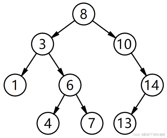
Python 数据结构
1.概念 数据结构是计算机科学中的一个核心概念,它是指数据的组织、管理和存储方式,以及数据元素之间的关系。数据结构通常用于允许高效的数据插入、删除和搜索操作。 数据结构大致分为几大类: 线性结构:数组、链表、栈、队列等…...
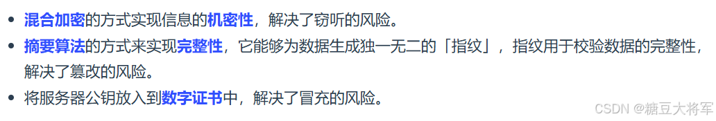
计算机网络八股文个人总结
1.TCP/IP模型和OSI模型的区别 在计算机网络中,TCP/IP 模型和 OSI 模型是两个重要的网络协议模型。它们帮助我们理解计算机通信的工作原理。以下是它们的主要区别,以通俗易懂的方式进行解释: 1. 模型层数 OSI 模型:有 7 层&#…...
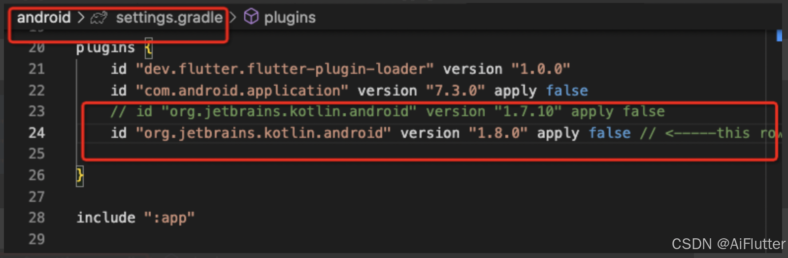
Flutter使用share_plus是提示发现了重复的类
问题描述 我现在下载了share_plus包后发现代码编译不通过,并提示Duplicate class kotlin.collections.jdk8.CollectionsJDK8Kt found in modules jetified-kotlin-stdlib-1.8.22 (org.jetbrains.kotlin:kotlin-stdlib:1.8.22) and jetified-kotlin-stdlib-jdk8-1.7…...

【Linux】编辑器vim 与 编译器gcc/g++
目录 一、编辑器vim: 1、对vim初步理解: 2、vim的模式: 3、进入与退出: 4、vim命令模式下的指令集: 移动光标: 删除: cv: 撤销: 其他: 5、vim底行模…...
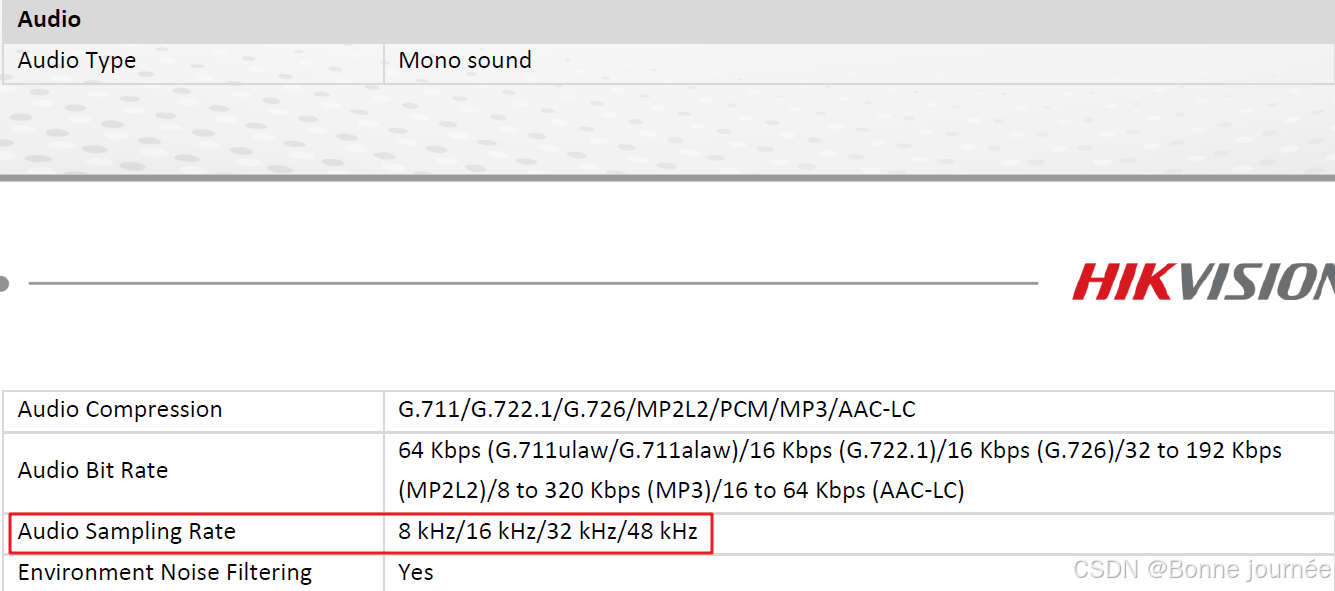
音频中sample rate是什么意思?
sample rate在数字信号处理中,指的是采样频率,即每秒钟从连续信号中抽取的样本数量。采样频率越高,信号的还原度越高,但同时也会增加计算负担和存储需求。 实际应用场景 在音频处理中,设置合适的采样率可以…...
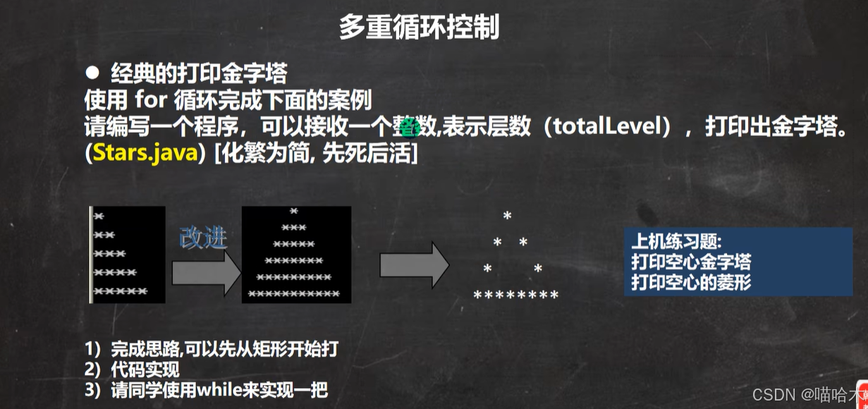
Java思想
学习韩老师的java课程 一步一步拆解需求,先写死的再写活的 首先我只是写了个输出一个*的程序 然后写了输出靠墙的1到n,n排n个的*符号输出程序 再写了加入空格的实心金字塔程序,最后写了这个镂空的金字塔 一下就是成品 import java.util.Sc…...

演练纪实丨 同创永益圆满完成10月份灾备切换演练支持
2024年10月,同创永益共支持5家客户圆满完成灾备切换演练,共涉及70多套核心系统总切换与回切步骤6000余个,成功率100%,RTO时长均达到客户要求。 其中耗时最短的一次演练仅花费约3个小时,共涉及32套系统的灾备切换演练&a…...

OpenAnolis峰会技术干货:从内核优化到云原生实战与开源参与
1. 项目概述:一场不容错过的技术盛宴如果你是一名长期耕耘在操作系统、云计算或基础软件领域的开发者或技术决策者,那么“2022全球开源峰会OpenAnolis分论坛”这个标题,对你而言绝不仅仅是一场普通的线上或线下会议通知。它更像是一份来自技术…...

Sunshine游戏串流:打造你自己的云端游戏主机
Sunshine游戏串流:打造你自己的云端游戏主机 【免费下载链接】Sunshine Self-hosted game stream host for Moonlight. 项目地址: https://gitcode.com/GitHub_Trending/su/Sunshine 想要在客厅大屏、卧室平板甚至手机上玩书房电脑里的3A大作吗?S…...

革命性AI背景移除:obs-backgroundremoval实现零绿幕专业级虚拟背景
革命性AI背景移除:obs-backgroundremoval实现零绿幕专业级虚拟背景 【免费下载链接】obs-backgroundremoval An OBS plugin for removing background in portrait images (video), making it easy to replace the background when recording or streaming. 项目地…...

YOLOv8模型家族全解析:P2、P6、标准版到底该选哪个?一张图帮你搞定选择困难症
YOLOv8模型家族全解析:P2、P6、标准版到底该选哪个? 在计算机视觉项目的初期,模型选型往往是最令人头疼的环节。面对GitHub仓库中琳琅满目的YAML配置文件,即便是经验丰富的工程师也难免陷入选择困难。YOLOv8作为当前最先进的目标检…...

智慧工业轮胎X光图像金属与结构缺陷检测数据集VOC+YOLO格式896张11类别
数据集格式:Pascal VOC格式YOLO格式(不包含分割路径的txt文件,仅仅包含jpg图片以及对应的VOC格式xml文件和yolo格式txt文件)图片数量(jpg文件个数):896标注数量(xml文件个数):896标注数量(txt文件个数):896标注类别数&…...

Go语言云原生开发:构建高可用微服务架构
Go语言云原生开发:构建高可用微服务架构 引言 云原生开发已成为现代应用开发的主流范式,Go语言凭借其轻量级、高性能和出色的并发支持,成为云原生开发的首选语言。本文将深入探讨Go语言在云原生环境中的应用,帮助您构建高可用的微…...

STM32图像识别实战:从传统CV到TinyML的边缘AI部署
1. 项目概述:当STM32遇上图像识别在嵌入式开发领域,STM32系列微控制器因其出色的性能、丰富的外设和极高的性价比,早已成为工程师和爱好者的“瑞士军刀”。从简单的LED闪烁到复杂的电机控制、通信协议栈,STM32几乎无所不能。但提到…...

RISC-V双芯架构在智慧燃气报警器中的系统级设计与工程实践
1. 项目概述:当RISC-V芯遇上智慧燃气最近在深圳的智慧燃气发展论坛上,我注意到一家叫微五科技的芯片设计公司,他们带来了一套挺有意思的解决方案。核心不是别的,正是当下在嵌入式领域越来越火的RISC-V架构。他们这次重点展示的&am…...

别再死记硬背了!用NestJS + TypeORM实战‘用户-标签’系统,搞懂OneToMany和ManyToOne
NestJS TypeORM实战:构建高可维护的用户标签系统 在开发内容管理平台时,用户与标签的关联关系是典型的多对一建模场景。本文将带你从零实现一个基于NestJS和TypeORM的生产级用户标签系统,重点解析OneToMany和ManyToOne在实际项目中的最佳实践…...

Gitee项目管理为什么成为中国团队首选:本土化、安全合规与DevOps全链路的三重优势
作者:DevOps效能研究团队 资料依据:Gitee官方数据(2025年Q2)、《2025中国开发者生态报告》、中国信息通信研究院DevOps能力成熟度评估报告 适读对象:技术负责人、项目经理、研发总监、企业CTO、数字化转型决策者 核心结…...