第12周:LSTM(火灾温度)
1.库以及数据的导入
1.1库的导入
import torch.nn.functional as F
import numpy  as np
import pandas as pd
import torch
from torch import nn
1.2数据集的导入
data = pd.read_csv("woodpine2.csv")data
| Time | Tem1 | CO 1 | Soot 1 | |
|---|---|---|---|---|
| 0 | 0.000 | 25.0 | 0.000000 | 0.000000 |
| 1 | 0.228 | 25.0 | 0.000000 | 0.000000 |
| 2 | 0.456 | 25.0 | 0.000000 | 0.000000 |
| 3 | 0.685 | 25.0 | 0.000000 | 0.000000 |
| 4 | 0.913 | 25.0 | 0.000000 | 0.000000 |
| ... | ... | ... | ... | ... |
| 5943 | 366.000 | 295.0 | 0.000077 | 0.000496 |
| 5944 | 366.000 | 294.0 | 0.000077 | 0.000494 |
| 5945 | 367.000 | 292.0 | 0.000077 | 0.000491 |
| 5946 | 367.000 | 291.0 | 0.000076 | 0.000489 |
| 5947 | 367.000 | 290.0 | 0.000076 | 0.000487 |
5948 rows × 4 columns
1.3数据集可视化
import matplotlib.pyplot as plt
import seaborn as snsplt.rcParams['savefig.dpi'] = 500 #图片像素
plt.rcParams['figure.dpi']  = 500 #分辨率fig, ax =plt.subplots(1,3,constrained_layout=True, figsize=(14, 3))sns.lineplot(data=data["Tem1"], ax=ax[0])
sns.lineplot(data=data["CO 1"], ax=ax[1])
sns.lineplot(data=data["Soot 1"], ax=ax[2])
plt.show()
](https://i-blog.csdnimg.cn/direct/eb1d674bdaea4502835e7b7489dc586f.png)
dataFrame = data.iloc[:,1:]
dataFrame
| Tem1 | CO 1 | Soot 1 | |
|---|---|---|---|
| 0 | 25.0 | 0.000000 | 0.000000 |
| 1 | 25.0 | 0.000000 | 0.000000 |
| 2 | 25.0 | 0.000000 | 0.000000 |
| 3 | 25.0 | 0.000000 | 0.000000 |
| 4 | 25.0 | 0.000000 | 0.000000 |
| ... | ... | ... | ... |
| 5943 | 295.0 | 0.000077 | 0.000496 |
| 5944 | 294.0 | 0.000077 | 0.000494 |
| 5945 | 292.0 | 0.000077 | 0.000491 |
| 5946 | 291.0 | 0.000076 | 0.000489 |
| 5947 | 290.0 | 0.000076 | 0.000487 |
5948 rows × 3 columns
2.数据集的构建
2.1数据的预处理
from sklearn.preprocessing import MinMaxScalerdataFrame = data.iloc[:,1:].copy()
sc  = MinMaxScaler(feature_range=(0, 1)) #将数据归一化,范围是0到1for i in ['CO 1', 'Soot 1', 'Tem1']:dataFrame[i] = sc.fit_transform(dataFrame[i].values.reshape(-1, 1))dataFrame.shape
(5948, 3)
2.设置X,y
width_X = 8
width_y = 1##取前8个时间段的Tem1、CO 1、Soot 1为X,第9个时间段的Tem1为y。
X = []
y = []in_start = 0for _, _ in data.iterrows():in_end  = in_start + width_Xout_end = in_end   + width_yif out_end < len(dataFrame):X_ = np.array(dataFrame.iloc[in_start:in_end , ])y_ = np.array(dataFrame.iloc[in_end  :out_end, 0])X.append(X_)y.append(y_)in_start += 1X = np.array(X)
y = np.array(y).reshape(-1,1,1)X.shape, y.shape
((5939, 8, 3), (5939, 1, 1))
#检查数据集中是否有空值
print(np.any(np.isnan(X)))
print(np.any(np.isnan(y)))
False
False
2.3划分数据集
X_train = torch.tensor(np.array(X[:5000]), dtype=torch.float32)
y_train = torch.tensor(np.array(y[:5000]), dtype=torch.float32)X_test  = torch.tensor(np.array(X[5000:]), dtype=torch.float32)
y_test  = torch.tensor(np.array(y[5000:]), dtype=torch.float32)
X_train.shape, y_train.shape
(torch.Size([5000, 8, 3]), torch.Size([5000, 1, 1]))
from torch.utils.data import TensorDataset, DataLoadertrain_dl = DataLoader(TensorDataset(X_train, y_train),batch_size=64, shuffle=False)test_dl = DataLoader(TensorDataset(X_test, y_test),batch_size=64, shuffle=False)
3.模型训练
3.1模型构建
class model_lstm(nn.Module):def __init__(self):super(model_lstm, self).__init__()self.lstm0 = nn.LSTM(input_size=3 ,hidden_size=320, num_layers=1, batch_first=True)self.lstm1 = nn.LSTM(input_size=320 ,hidden_size=320, num_layers=1, batch_first=True)self.fc0   = nn.Linear(320, 1)def forward(self, x):out, hidden1 = self.lstm0(x) out, _ = self.lstm1(out, hidden1) out    = self.fc0(out) return out[:, -1:, :]   #取2个预测值,否则经过lstm会得到8*2个预测model = model_lstm()
model
model_lstm((lstm0): LSTM(3, 320, batch_first=True)(lstm1): LSTM(320, 320, batch_first=True)(fc0): Linear(in_features=320, out_features=1, bias=True)
)
model(torch.rand(30,8,3)).shape
torch.Size([30, 1, 1])
3.2定义训练函数
# 训练循环
import copy
def train(train_dl, model, loss_fn, opt, lr_scheduler=None):size        = len(train_dl.dataset)  num_batches = len(train_dl)   train_loss  = 0  # 初始化训练损失和正确率for x, y in train_dl:  x, y = x.to(device), y.to(device)# 计算预测误差pred = model(x)          # 网络输出loss = loss_fn(pred, y)  # 计算网络输出和真实值之间的差距# 反向传播opt.zero_grad()  # grad属性归零loss.backward()  # 反向传播opt.step()       # 每一步自动更新# 记录losstrain_loss += loss.item()if lr_scheduler is not None:lr_scheduler.step()print("learning rate = {:.5f}".format(opt.param_groups[0]['lr']), end="  ")train_loss /= num_batchesreturn train_loss
3.3定义测试函数
def test (dataloader, model, loss_fn):size = len(dataloader.dataset) # 测试集的大小num_batches = len(dataloader) # 批次数目test_loss = 0# 当不进行训练时,停止梯度更新,节省计算内存消耗with torch.no_grad():for x, y in dataloader:x, y = x.to(device), y.to(device)# 计算lossy_pred = model(x)loss = loss_fn(y_pred, y)test_loss += loss.item()test_loss /= num_batchesreturn test_loss
#设置GPU训练
device=torch.device("cuda" if torch.cuda.is_available() else "cpu")
device
device(type='cpu')
3.4正式训练模型
#训练模型
model = model_lstm()
model = model.to(device)
loss_fn    = nn.MSELoss() # 创建损失函数
learn_rate = 1e-1   # 学习率
opt        = torch.optim.SGD(model.parameters(),lr=learn_rate,weight_decay=1e-4)
epochs     = 50
train_loss = []
test_loss  = []
lr_scheduler = torch.optim.lr_scheduler.CosineAnnealingLR(opt,epochs, last_epoch=-1) for epoch in range(epochs):model.train()epoch_train_loss = train(train_dl, model, loss_fn, opt, lr_scheduler)model.eval()epoch_test_loss = test(test_dl, model, loss_fn)train_loss.append(epoch_train_loss)test_loss.append(epoch_test_loss)template = ('Epoch:{:2d}, Train_loss:{:.5f}, Test_loss:{:.5f}')print(template.format(epoch+1, epoch_train_loss,  epoch_test_loss))print("="*20, 'Done', "="*20)
learning rate = 0.09990  Epoch: 1, Train_loss:0.00131, Test_loss:0.01243
learning rate = 0.09961  Epoch: 2, Train_loss:0.01428, Test_loss:0.01208
learning rate = 0.09911  Epoch: 3, Train_loss:0.01401, Test_loss:0.01172
learning rate = 0.09843  Epoch: 4, Train_loss:0.01369, Test_loss:0.01132
learning rate = 0.09755  Epoch: 5, Train_loss:0.01333, Test_loss:0.01088
learning rate = 0.09649  Epoch: 6, Train_loss:0.01289, Test_loss:0.01039
learning rate = 0.09524  Epoch: 7, Train_loss:0.01237, Test_loss:0.00983
learning rate = 0.09382  Epoch: 8, Train_loss:0.01174, Test_loss:0.00919
learning rate = 0.09222  Epoch: 9, Train_loss:0.01100, Test_loss:0.00849
learning rate = 0.09045  Epoch:10, Train_loss:0.01015, Test_loss:0.00772
learning rate = 0.08853  Epoch:11, Train_loss:0.00918, Test_loss:0.00689
learning rate = 0.08645  Epoch:12, Train_loss:0.00812, Test_loss:0.00604
learning rate = 0.08423  Epoch:13, Train_loss:0.00701, Test_loss:0.00520
learning rate = 0.08187  Epoch:14, Train_loss:0.00588, Test_loss:0.00438
learning rate = 0.07939  Epoch:15, Train_loss:0.00479, Test_loss:0.00363
learning rate = 0.07679  Epoch:16, Train_loss:0.00379, Test_loss:0.00297
learning rate = 0.07409  Epoch:17, Train_loss:0.00291, Test_loss:0.00241
learning rate = 0.07129  Epoch:18, Train_loss:0.00219, Test_loss:0.00196
learning rate = 0.06841  Epoch:19, Train_loss:0.00161, Test_loss:0.00160
learning rate = 0.06545  Epoch:20, Train_loss:0.00117, Test_loss:0.00133
learning rate = 0.06243  Epoch:21, Train_loss:0.00084, Test_loss:0.00112
learning rate = 0.05937  Epoch:22, Train_loss:0.00061, Test_loss:0.00098
learning rate = 0.05627  Epoch:23, Train_loss:0.00045, Test_loss:0.00087
learning rate = 0.05314  Epoch:24, Train_loss:0.00034, Test_loss:0.00079
learning rate = 0.05000  Epoch:25, Train_loss:0.00027, Test_loss:0.00073
learning rate = 0.04686  Epoch:26, Train_loss:0.00021, Test_loss:0.00069
learning rate = 0.04373  Epoch:27, Train_loss:0.00018, Test_loss:0.00066
learning rate = 0.04063  Epoch:28, Train_loss:0.00016, Test_loss:0.00063
learning rate = 0.03757  Epoch:29, Train_loss:0.00014, Test_loss:0.00061
learning rate = 0.03455  Epoch:30, Train_loss:0.00013, Test_loss:0.00060
learning rate = 0.03159  Epoch:31, Train_loss:0.00012, Test_loss:0.00058
learning rate = 0.02871  Epoch:32, Train_loss:0.00012, Test_loss:0.00058
learning rate = 0.02591  Epoch:33, Train_loss:0.00012, Test_loss:0.00057
learning rate = 0.02321  Epoch:34, Train_loss:0.00012, Test_loss:0.00057
learning rate = 0.02061  Epoch:35, Train_loss:0.00012, Test_loss:0.00057
learning rate = 0.01813  Epoch:36, Train_loss:0.00012, Test_loss:0.00057
learning rate = 0.01577  Epoch:37, Train_loss:0.00012, Test_loss:0.00057
learning rate = 0.01355  Epoch:38, Train_loss:0.00012, Test_loss:0.00057
learning rate = 0.01147  Epoch:39, Train_loss:0.00013, Test_loss:0.00058
learning rate = 0.00955  Epoch:40, Train_loss:0.00013, Test_loss:0.00059
learning rate = 0.00778  Epoch:41, Train_loss:0.00013, Test_loss:0.00060
learning rate = 0.00618  Epoch:42, Train_loss:0.00014, Test_loss:0.00061
learning rate = 0.00476  Epoch:43, Train_loss:0.00014, Test_loss:0.00061
learning rate = 0.00351  Epoch:44, Train_loss:0.00014, Test_loss:0.00062
learning rate = 0.00245  Epoch:45, Train_loss:0.00014, Test_loss:0.00062
learning rate = 0.00157  Epoch:46, Train_loss:0.00014, Test_loss:0.00062
learning rate = 0.00089  Epoch:47, Train_loss:0.00014, Test_loss:0.00062
learning rate = 0.00039  Epoch:48, Train_loss:0.00014, Test_loss:0.00062
learning rate = 0.00010  Epoch:49, Train_loss:0.00014, Test_loss:0.00062
learning rate = 0.00000  Epoch:50, Train_loss:0.00014, Test_loss:0.00062
==================== Done ====================
4.模型评估
4.1loss
import matplotlib.pyplot as plt
from datetime import datetime
current_time = datetime.now() # 获取当前时间plt.figure(figsize=(5, 3),dpi=120)plt.plot(train_loss    , label='LSTM Training Loss')
plt.plot(test_loss, label='LSTM Validation Loss')plt.title('Training and Validation Loss')
plt.xlabel(current_time) # 打卡请带上时间戳,否则代码截图无效
plt.legend()
plt.show()

4.2模型调用及预测
predicted_y_lstm = sc.inverse_transform(model(X_test).detach().numpy().reshape(-1,1))                    # 测试集输入模型进行预测
y_test_1         = sc.inverse_transform(y_test.reshape(-1,1))
y_test_one       = [i[0] for i in y_test_1]
predicted_y_lstm_one = [i[0] for i in predicted_y_lstm]plt.figure(figsize=(5, 3),dpi=120)
# 画出真实数据和预测数据的对比曲线
plt.plot(y_test_one[:2000], color='red', label='real_temp')
plt.plot(predicted_y_lstm_one[:2000], color='blue', label='prediction')plt.title('Title')
plt.xlabel('X')
plt.ylabel('Y')
plt.legend()
plt.show()

4.3R2值评估
from sklearn import metrics
"""
RMSE :均方根误差  ----->  对均方误差开方
R2   :决定系数,可以简单理解为反映模型拟合优度的重要的统计量
"""
RMSE_lstm  = metrics.mean_squared_error(predicted_y_lstm_one, y_test_1)**0.5
R2_lstm    = metrics.r2_score(predicted_y_lstm_one, y_test_1)print('均方根误差: %.5f' % RMSE_lstm)
print('R2: %.5f' % R2_lstm)
均方根误差: 7.07942
R2: 0.82427
- 🍨 本文为🔗365天深度学习训练营 中的学习记录博客
- *🍖 原作者:K同学啊
相关文章:
第12周:LSTM(火灾温度)
1.库以及数据的导入 1.1库的导入 import torch.nn.functional as F import numpy as np import pandas as pd import torch from torch import nn1.2数据集的导入 data pd.read_csv("woodpine2.csv")dataTimeTem1CO 1Soot 100.00025.00.0000000.00000010.22825.…...

MySQL的SQL执行流程
项目查询数据库的流程 用户通过Tomcat服务器发送请求到MySQL数据库的过程。 用户发起请求:用户通过浏览器或其他客户端向Tomcat服务器发送HTTP请求。 Tomcat服务器处理请求: Tomcat服务器接收用户的请求,并创建一个线程来处理这个请求。 线…...

Foundation CSS 可见性
Foundation CSS 可见性 引言 在网页设计中,CSS可见性是一个至关重要的概念。它决定了元素在网页上是否可见,以及如何显示。Foundation CSS 是一个流行的前端框架,它提供了丰富的工具和组件来帮助开发者构建响应式和可访问的网页。本文将深入探讨 Foundation CSS 中的可见性…...

7. Docker 容器数据卷的使用(超详细的讲解说明)
7. Docker 容器数据卷的使用(超详细的讲解说明) 文章目录 7. Docker 容器数据卷的使用(超详细的讲解说明)1. Docker容器数据卷概述2. Docker 容器数据卷的使用演示:2.1 宿主 和 容器之间映射添加容器卷2.2 容器数据卷 读写规则映射添加说明2.3 容器数据卷的继承和共…...
算法——结合实例了解广度优先搜索(BFS)搜索
一、广度优先搜索初印象 想象一下,你身处一座陌生的城市,想要从当前位置前往某个景点,你打开手机上的地图导航软件,输入目的地后,导航软件会迅速规划出一条最短路线。这背后,就可能运用到了广度优先搜索&am…...

qt QCommandLineOption 详解
1、概述 QCommandLineOption类是Qt框架中用于解析命令行参数的类。它提供了一种方便的方式来定义和解析命令行选项,并且可以与QCommandLineParser类一起使用,以便在应用程序中轻松处理命令行参数。通过QCommandLineOption类,开发者可以更便捷…...

Linux权限提升-内核溢出
一:Web到Linux-内核溢出Dcow 复现环境:https://www.vulnhub.com/entry/lampiao-1,249/ 1.信息收集:探测⽬标ip及开发端⼝ 2.Web漏洞利⽤: 查找drupal相关漏洞 search drupal # 进⾏漏洞利⽤ use exploit/unix/webapp/drupal_dr…...

【环境安装】重装Docker-26.0.2版本
【机器背景说明】Linux-Centos7;已有低版本的Docker 【目标环境说明】 卸载已有Docker,用docker-26.0.2.tgz安装包安装 1.Docker包下载 下载地址:Index of linux/static/stable/x86_64/ 2.卸载已有的Docker 卸载之前首先停掉服务 sudo…...

【云安全】云原生- K8S API Server 未授权访问
API Server 是 Kubernetes 集群的核心管理接口,所有资源请求和操作都通过 kube-apiserver 提供的 API 进行处理。默认情况下,API Server 会监听两个端口:8080 和 6443。如果配置不当,可能会导致未授权访问的安全风险。 8080 端口…...

笔记7——条件判断
条件判断 主要通过 if、elif 和 else 语句来实现 语法结构 # if 条件1: # 条件1为真时执行的代码 # elif 条件2: # 条件1为假、且条件2为真时执行的代码 # elif 条件3: # 条件1、2为假、且条件3为真时执行的代码 # ... # else: # 所…...

Word 公式转 CSDN 插件 发布
经过几个月的苦修,这款插件终于面世了。 从Word复制公式到CSDN粘贴,总是出现公式中的文字被单独提出来,而公式作为一个图片被粘贴的情况。公式多了的时候还会导致CSDN禁止进一步的上传公式。 经过对CSDN公式的研究,发现在粘贴公…...

二次封装axios解决异步通信痛点
为了方便扩展,和增加配置的灵活性,这里将通过封装一个类来实现axios的二次封装,要实现的功能包括: 为请求传入自定义的配置,控制单次请求的不同行为在响应拦截器中对业务逻辑进行处理,根据业务约定的成功数据结构,返回业务数据对响应错误进行处理,配置显示对话框或消息形…...

算法——结合实例了解深度优先搜索(DFS)
一,深度优先搜索(DFS)详解 DFS是什么? 深度优先搜索(Depth-First Search,DFS)是一种用于遍历或搜索树、图的算法。其核心思想是尽可能深地探索分支,直到无法继续时回溯到上一个节点…...
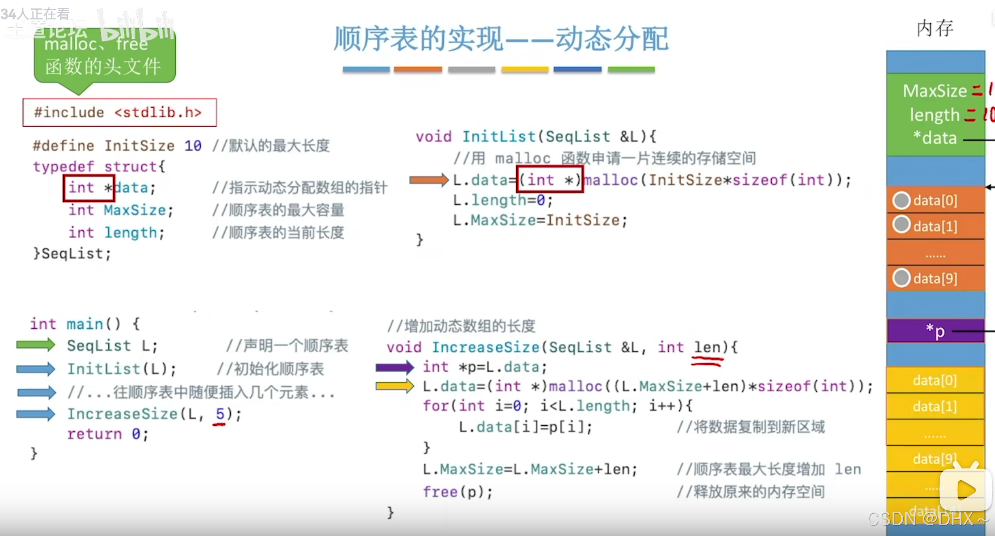
数据结构(考研)
线性表 顺序表 顺序表的静态分配 //线性表的元素类型为 ElemType//顺序表的静态分配 #define MaxSize10 typedef int ElemType; typedef struct{ElemType data[MaxSize];int length; }SqList;顺序表的动态分配 //顺序表的动态分配 #define InitSize 10 typedef struct{El…...

使用SSE协议进行服务端向客户端主动发送消息
1.创建一个SSE配置类: 1.1代码如下:package com.campus.platform.config;import org.springframework.context.annotation.Bean; import org.springframework.context.annotation.Configuration; import org.springframework.web.servlet.config.annotation.AsyncS…...

FastAPI 高并发与性能优化
FastAPI 高并发与性能优化 目录 🚀 高并发应用设计原则🧑💻 异步 I/O 优化 Web 服务响应速度⏳ 在 FastAPI 中优化异步任务执行顺序🔒 高并发中的共享资源与线程安全问题 1. 🚀 高并发应用设计原则 在构建高并发应…...

DFS+回溯+剪枝(深度优先搜索)——搜索算法
目录 一、递归 1.什么是递归? 2.什么时候使用递归? 3.如何理解递归? 4.如何写好递归? 二、记忆化搜索(记忆递归) 三、回溯 四、剪枝 五、综合试题 1.N皇后 2.解数独 DFS也就是深度优先搜索&am…...
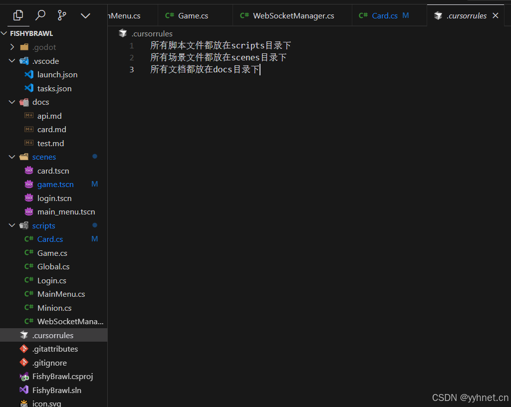
在cursor/vscode中使用godot C#进行游戏开发
要在 Visual Studio Code(VS Code)中启动 C#Godot 项目,可以按照以下步骤进行配置: 1.安装必要的工具 • 安装 Visual Studio Code:确保你已经安装了最新版本的 VS Code。 • 安装.NET SDK:下载并安装.NET 7.x SDK(…...

vant4 van-list组件的使用
<van-listv-if"joblist && joblist.length > 0"v-model:loading"loading":finished"finished":immediate-check"false"finished-text"没有更多了"load"onLoad">// 加载 const loading ref(fals…...

介绍 Liquibase、Flyway、Talend 和 Apache NiFi:选择适合的工具
在现代软件开发中,尤其是在数据库管理和数据集成方面,选择合适的工具至关重要。本文将介绍四个流行的工具:Liquibase、Flyway、Talend 和 Apache NiFi,分析它们的应用、依赖以及如何选择适合的工具。 1. Liquibase 简介ÿ…...

开发者技能日志工具:用CLI与SQLite构建个人技术成长追踪系统
1. 项目概述:一个技能日志记录器的诞生 最近在整理自己的技术栈和项目经验时,我遇到了一个很多开发者都有的痛点:学了那么多东西,做了那么多项目,但真要写简历或者回顾成长路径时,记忆总是模糊的。今天学了…...

为什么选择update-golang:5大优势对比传统安装方式
为什么选择update-golang:5大优势对比传统安装方式 【免费下载链接】update-golang update-golang is a script to easily fetch and install new Golang releases with minimum system intrusion 项目地址: https://gitcode.com/gh_mirrors/up/update-golang …...

BepInEx IL2CPP启动失败终极解决指南:从异常诊断到游戏正常运行
BepInEx IL2CPP启动失败终极解决指南:从异常诊断到游戏正常运行 【免费下载链接】BepInEx Unity / XNA game patcher and plugin framework 项目地址: https://gitcode.com/GitHub_Trending/be/BepInEx BepInEx作为Unity游戏插件框架,为玩家和开发…...

虚拟原型技术:软硬件协同开发与多核处理器调试新范式
1. 虚拟原型平台:从芯片设计到软件集成的范式转变在嵌入式系统开发领域,尤其是涉及复杂多核处理器的项目里,一个长期存在的“鸡生蛋还是蛋生鸡”的困境一直困扰着工程师们:硬件原型板(EVB)尚未就绪…...

LobsterPress v5.0:为AI Agent构建长期记忆系统的架构与实践
1. 项目概述:为AI Agent构建“数字海马体”如果你和我一样,长期与ChatGPT、Claude这类大语言模型打交道,一定会被一个核心问题困扰:它们记性太差了。无论你昨天花了多少时间与AI深入探讨一个项目细节,今天开启新对话时…...

大语言模型评测框架解析:从公平对比到工程选型实践
1. 项目概述与核心价值最近在GitHub上看到一个挺有意思的项目,叫“ai-llm-comparison”。光看名字,你大概能猜到它是做什么的——对比不同的大语言模型。但如果你以为这只是个简单的跑分列表,那就太小看它了。作为一个在AI应用开发领域摸爬滚…...

基于RAG与LangChain的法律AI助手:从技术原理到开源实践
1. 项目概述:当AI遇上法律,一个开源法律智能助手的诞生最近几年,AI大模型的热潮席卷了各行各业,从写代码到画图,从客服到教育,似乎没有哪个领域能置身事外。作为一名在技术圈摸爬滚打多年的从业者ÿ…...

AI绘画自动化:从批量生成到Pixiv发布的半自动工具实践
1. 项目概述:从手动到自动,解放AI绘画生产力的全流程工具 如果你是一名深度使用NovelAI或Stable Diffusion这类AI绘画工具的创作者,那么你一定对“批量生成”和“自动发布”这两个词背后的痛楚深有体会。每次生成图片,你都需要在W…...

终极指南:如何用NPYViewer快速可视化NumPy数组数据
终极指南:如何用NPYViewer快速可视化NumPy数组数据 【免费下载链接】NPYViewer Load and view .npy files containing 2D and 1D NumPy arrays. 项目地址: https://gitcode.com/gh_mirrors/np/NPYViewer 还在为NumPy数组数据可视化而烦恼吗?面对二…...

三步永久保存微信聊天记录的完整指南:告别数据丢失的烦恼
三步永久保存微信聊天记录的完整指南:告别数据丢失的烦恼 【免费下载链接】WeChatMsg 提取微信聊天记录,将其导出成HTML、Word、CSV文档永久保存,对聊天记录进行分析生成年度聊天报告 项目地址: https://gitcode.com/GitHub_Trending/we/We…...