2025-06-08-深度学习网络介绍(语义分割,实例分割,目标检测)
深度学习网络介绍(语义分割,实例分割,目标检测)
前言
在开始这篇文章之前,我们得首先弄明白,什么是图像分割?
我们知道一个图像只不过是许多像素的集合。图像分割分类是对图像中属于特定类别的像素进行分类的过程,即像素级别的下游任务。因此图像分割简单来说就是按像素进行分类的问题。
传统的图像分割算法均是基于灰度值的不连续和相似的性质。而基于深度学习的图像分割技术则是利用卷积神经网络,来理解图像中的每个像素所代表的真实世界物体,这在以前是难以想象的。
语义分割(Semantic Segmentation)
定义
“语义”是个很抽象的概念,在 2D 图像领域,每个像素点作为最小单位,它的像素值代表的就是一个特征,即“语义”信息。语义分割会为图像中的每个像素分配一个类别,但是同一类别之间的对象不会区分。而实例分割,只对特定的物体进行分类。这看起来与目标检测相似,不同的是目标检测输出目标的边界框和类别,实例分割输出的是目标的 Mask 和类别。具体而言,语义分割的目的是为了从像素级别理解图像的内容,并为图像中的每个像素分配一个对象类。
语义分割是一种将图像中的每个像素分配给特定类别的技术。其目标是识别图像中存在的各种对象和背景,并为每个像素分配相应的类别标签。例如,将图像中的像素划分为人、树、草地和天空等不同区域。是图像处理和机器视觉一个重要分支。与分类任务不同,语义分割需要判断图像每个像素点的类别,进行精确分割。语义分割目前在自动驾驶、自动抠图、医疗影像等领域有着比较广泛的应用。
特点
- 提供精确的像素级分类,有助于深入理解图像内容。
- 无法区分同一类别中的不同实例。
语义分割的应用
语义分割在多个领域有广泛应用:
- 自动驾驶:用于道路、车辆和行人的识别。
- 医学成像:用于组织和器官的分割。
- 卫星遥感:用于土地覆盖分类。
常见模型
FCN(Fully Convolutional Network)
- 优点:简单易用,但是现在已经很少使用了,但它的历史贡献不可忽视。
- 缺点:分割精度较低,可能无法很好地处理细节。
提出初衷
FCN(全卷积网络)模型的初衷是为了解决传统卷积神经网络(CNN)在语义分割任务中的局限性。具体而言,传统 CNN 使用全连接层进行分类,这会丢失图像的空间位置信息,导致其不适合像素级的预测任务。FCN 的核心动机包括:
- 实现端到端的像素级预测:FCN 通过将全连接层替换为卷积层,使得网络能够接受任意尺寸的输入图像,并输出与输入尺寸相同的像素级预测结果。
- 保留空间信息:取消全连接层后,FCN 能够保留图像的空间位置信息,从而更好地适应语义分割任务。
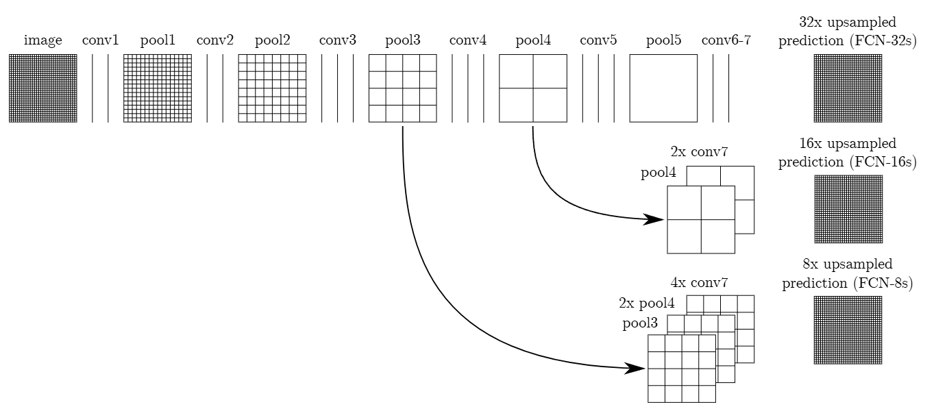
- 提高分割效率和精度:通过引入反卷积层(上采样层)和跳跃连接(Skip Connections),FCN 能够融合不同深度的特征,兼顾全局语义信息和局部细节,从而提升分割精度。
- 利用预训练模型加速训练:FCN 可以基于预训练的分类模型(如 AlexNet、VGG 等)进行微调,从而显著加速训练过程并提高模型性能。
网络结构
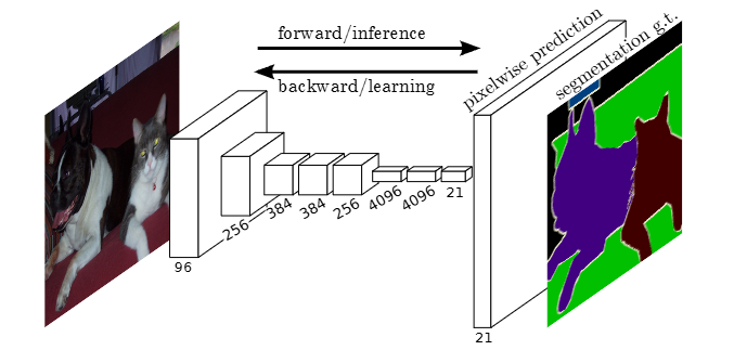
通常 CNN 网络在卷积层之后会接上若干个全连接层, 将卷积层产生的特征图(feature map)映射成一个固定长度的特征向量。以 AlexNet 为代表的经典 CNN 结构适合于图像级的分类和回归任务,因为它们最后都期望得到整个输入图像的一个数值描述(概率)。
FCN 对图像进行像素级的分类,从而解决了语义级别的图像分割(semantic segmentation)问题。与经典的 CNN 在卷积层之后使用全连接层得到固定长度的特征向量进行分类(全连接层 +softmax 输出)不同,FCN 可以接受任意尺寸的输入图像,采用反卷积层对最后一个卷积层的 feature map 进行上采样, 使它恢复到输入图像相同的尺寸,从而可以对每个像素都产生了一个预测, 同时保留了原始输入图像中的空间信息, 最后在上采样的特征图上进行逐像素分类。
FCN(全卷积网络)为了解决语义分割(semantic segmentation)问题而提出,它对图像进行像素级的分类,能够保留原始输入图像中的空间信息。与传统 CNN 不同,FCN 可以接受任意尺寸的输入图像,并通过以下方式实现像素级分类:
- 去除全连接层:FCN 将传统 CNN 中的全连接层替换为卷积层,从而保留空间信息。
- 上采样操作:使用反卷积层(上采样层)对最后一个卷积层的特征图进行上采样,恢复到与输入图像相同的尺寸。
- 逐像素分类:在上采样后的特征图上进行逐像素分类,为每个像素生成类别预测。
Q:FCN 是如何通过上采样操作恢复特征图的空间分辨率的?
模型代码
论文源码
import caffe
from caffe import layers as L, params as P
from caffe.coord_map import cropdef conv_relu(bottom, nout, ks=3, stride=1, pad=1):conv = L.Convolution(bottom, kernel_size=ks, stride=stride,num_output=nout, pad=pad,param=[dict(lr_mult=1, decay_mult=1), dict(lr_mult=2, decay_mult=0)])return conv, L.ReLU(conv, in_place=True)def max_pool(bottom, ks=2, stride=2):return L.Pooling(bottom, pool=P.Pooling.MAX, kernel_size=ks, stride=stride)def fcn(split):n = caffe.NetSpec()pydata_params = dict(split=split, mean=(104.00699, 116.66877, 122.67892),seed=1337)if split == 'train':pydata_params['sbdd_dir'] = '../data/sbdd/dataset'pylayer = 'SBDDSegDataLayer'else:pydata_params['voc_dir'] = '../data/pascal/VOC2011'pylayer = 'VOCSegDataLayer'n.data, n.label = L.Python(module='voc_layers', layer=pylayer,ntop=2, param_str=str(pydata_params))# the base netn.conv1_1, n.relu1_1 = conv_relu(n.data, 64, pad=100)n.conv1_2, n.relu1_2 = conv_relu(n.relu1_1, 64)n.pool1 = max_pool(n.relu1_2)n.conv2_1, n.relu2_1 = conv_relu(n.pool1, 128)n.conv2_2, n.relu2_2 = conv_relu(n.relu2_1, 128)n.pool2 = max_pool(n.relu2_2)n.conv3_1, n.relu3_1 = conv_relu(n.pool2, 256)n.conv3_2, n.relu3_2 = conv_relu(n.relu3_1, 256)n.conv3_3, n.relu3_3 = conv_relu(n.relu3_2, 256)n.pool3 = max_pool(n.relu3_3)n.conv4_1, n.relu4_1 = conv_relu(n.pool3, 512)n.conv4_2, n.relu4_2 = conv_relu(n.relu4_1, 512)n.conv4_3, n.relu4_3 = conv_relu(n.relu4_2, 512)n.pool4 = max_pool(n.relu4_3)n.conv5_1, n.relu5_1 = conv_relu(n.pool4, 512)n.conv5_2, n.relu5_2 = conv_relu(n.relu5_1, 512)n.conv5_3, n.relu5_3 = conv_relu(n.relu5_2, 512)n.pool5 = max_pool(n.relu5_3)# fully convn.fc6, n.relu6 = conv_relu(n.pool5, 4096, ks=7, pad=0)n.drop6 = L.Dropout(n.relu6, dropout_ratio=0.5, in_place=True)n.fc7, n.relu7 = conv_relu(n.drop6, 4096, ks=1, pad=0)n.drop7 = L.Dropout(n.relu7, dropout_ratio=0.5, in_place=True)n.score_fr = L.Convolution(n.drop7, num_output=21, kernel_size=1, pad=0,param=[dict(lr_mult=1, decay_mult=1), dict(lr_mult=2, decay_mult=0)])n.upscore2 = L.Deconvolution(n.score_fr,convolution_param=dict(num_output=21, kernel_size=4, stride=2,bias_term=False),param=[dict(lr_mult=0)])n.score_pool4 = L.Convolution(n.pool4, num_output=21, kernel_size=1, pad=0,param=[dict(lr_mult=1, decay_mult=1), dict(lr_mult=2, decay_mult=0)])n.score_pool4c = crop(n.score_pool4, n.upscore2)n.fuse_pool4 = L.Eltwise(n.upscore2, n.score_pool4c,operation=P.Eltwise.SUM)n.upscore_pool4 = L.Deconvolution(n.fuse_pool4,convolution_param=dict(num_output=21, kernel_size=4, stride=2,bias_term=False),param=[dict(lr_mult=0)])n.score_pool3 = L.Convolution(n.pool3, num_output=21, kernel_size=1, pad=0,param=[dict(lr_mult=1, decay_mult=1), dict(lr_mult=2, decay_mult=0)])n.score_pool3c = crop(n.score_pool3, n.upscore_pool4)n.fuse_pool3 = L.Eltwise(n.upscore_pool4, n.score_pool3c,operation=P.Eltwise.SUM)n.upscore8 = L.Deconvolution(n.fuse_pool3,convolution_param=dict(num_output=21, kernel_size=16, stride=8,bias_term=False),param=[dict(lr_mult=0)])n.score = crop(n.upscore8, n.data)n.loss = L.SoftmaxWithLoss(n.score, n.label,loss_param=dict(normalize=False, ignore_label=255))return n.to_proto()def make_net():with open('train.prototxt', 'w') as f:f.write(str(fcn('train')))with open('val.prototxt', 'w') as f:f.write(str(fcn('seg11valid')))if __name__ == '__main__':make_net()
fcn8_vgg
from __future__ import absolute_import
from __future__ import division
from __future__ import print_functionimport os
import logging
from math import ceil
import sysimport numpy as np
import tensorflow as tfVGG_MEAN = [103.939, 116.779, 123.68]class FCN8VGG:def __init__(self, vgg16_npy_path=None):if vgg16_npy_path is None:path = sys.modules[self.__class__.__module__].__file__# print pathpath = os.path.abspath(os.path.join(path, os.pardir))# print pathpath = os.path.join(path, "vgg16.npy")vgg16_npy_path = pathlogging.info("Load npy file from '%s'.", vgg16_npy_path)if not os.path.isfile(vgg16_npy_path):logging.error(("File '%s' not found. Download it from ""ftp://mi.eng.cam.ac.uk/pub/mttt2/""models/vgg16.npy"), vgg16_npy_path)sys.exit(1)self.data_dict = np.load(vgg16_npy_path, encoding='latin1').item()self.wd = 5e-4print("npy file loaded")def build(self, rgb, train=False, num_classes=20, random_init_fc8=False,debug=False, use_dilated=False):"""Build the VGG model using loaded weightsParameters----------rgb: image batch tensorImage in rgb shap. Scaled to Intervall [0, 255]train: boolWhether to build train or inference graphnum_classes: intHow many classes should be predicted (by fc8)random_init_fc8 : boolWhether to initialize fc8 layer randomly.Finetuning is required in this case.debug: boolWhether to print additional Debug Information."""# Convert RGB to BGRwith tf.name_scope('Processing'):red, green, blue = tf.split(rgb, 3, 3)# assert red.get_shape().as_list()[1:] == [224, 224, 1]# assert green.get_shape().as_list()[1:] == [224, 224, 1]# assert blue.get_shape().as_list()[1:] == [224, 224, 1]bgr = tf.concat([blue - VGG_MEAN[0],green - VGG_MEAN[1],red - VGG_MEAN[2],], 3)if debug:bgr = tf.Print(bgr, [tf.shape(bgr)],message='Shape of input image: ',summarize=4, first_n=1)self.conv1_1 = self._conv_layer(bgr, "conv1_1")self.conv1_2 = self._conv_layer(self.conv1_1, "conv1_2")self.pool1 = self._max_pool(self.conv1_2, 'pool1', debug)self.conv2_1 = self._conv_layer(self.pool1, "conv2_1")self.conv2_2 = self._conv_layer(self.conv2_1, "conv2_2")self.pool2 = self._max_pool(self.conv2_2, 'pool2', debug)self.conv3_1 = self._conv_layer(self.pool2, "conv3_1")self.conv3_2 = self._conv_layer(self.conv3_1, "conv3_2")self.conv3_3 = self._conv_layer(self.conv3_2, "conv3_3")self.pool3 = self._max_pool(self.conv3_3, 'pool3', debug)self.conv4_1 = self._conv_layer(self.pool3, "conv4_1")self.conv4_2 = self._conv_layer(self.conv4_1, "conv4_2")self.conv4_3 = self._conv_layer(self.conv4_2, "conv4_3")if use_dilated:pad = [[0, 0], [0, 0]]self.pool4 = tf.nn.max_pool(self.conv4_3, ksize=[1, 2, 2, 1],strides=[1, 1, 1, 1],padding='SAME', name='pool4')self.pool4 = tf.space_to_batch(self.pool4,paddings=pad, block_size=2)else:self.pool4 = self._max_pool(self.conv4_3, 'pool4', debug)self.conv5_1 = self._conv_layer(self.pool4, "conv5_1")self.conv5_2 = self._conv_layer(self.conv5_1, "conv5_2")self.conv5_3 = self._conv_layer(self.conv5_2, "conv5_3")if use_dilated:pad = [[0, 0], [0, 0]]self.pool5 = tf.nn.max_pool(self.conv5_3, ksize=[1, 2, 2, 1],strides=[1, 1, 1, 1],padding='SAME', name='pool5')self.pool5 = tf.space_to_batch(self.pool5,paddings=pad, block_size=2)else:self.pool5 = self._max_pool(self.conv5_3, 'pool5', debug)self.fc6 = self._fc_layer(self.pool5, "fc6")if train:self.fc6 = tf.nn.dropout(self.fc6, 0.5)self.fc7 = self._fc_layer(self.fc6, "fc7")if train:self.fc7 = tf.nn.dropout(self.fc7, 0.5)if use_dilated:self.pool5 = tf.batch_to_space(self.pool5, crops=pad, block_size=2)self.pool5 = tf.batch_to_space(self.pool5, crops=pad, block_size=2)self.fc7 = tf.batch_to_space(self.fc7, crops=pad, block_size=2)self.fc7 = tf.batch_to_space(self.fc7, crops=pad, block_size=2)returnif random_init_fc8:self.score_fr = self._score_layer(self.fc7, "score_fr",num_classes)else:self.score_fr = self._fc_layer(self.fc7, "score_fr",num_classes=num_classes,relu=False)self.pred = tf.argmax(self.score_fr, dimension=3)self.upscore2 = self._upscore_layer(self.score_fr,shape=tf.shape(self.pool4),num_classes=num_classes,debug=debug, name='upscore2',ksize=4, stride=2)self.score_pool4 = self._score_layer(self.pool4, "score_pool4",num_classes=num_classes)self.fuse_pool4 = tf.add(self.upscore2, self.score_pool4)self.upscore4 = self._upscore_layer(self.fuse_pool4,shape=tf.shape(self.pool3),num_classes=num_classes,debug=debug, name='upscore4',ksize=4, stride=2)self.score_pool3 = self._score_layer(self.pool3, "score_pool3",num_classes=num_classes)self.fuse_pool3 = tf.add(self.upscore4, self.score_pool3)self.upscore32 = self._upscore_layer(self.fuse_pool3,shape=tf.shape(bgr),num_classes=num_classes,debug=debug, name='upscore32',ksize=16, stride=8)self.pred_up = tf.argmax(self.upscore32, dimension=3)def _max_pool(self, bottom, name, debug):pool = tf.nn.max_pool(bottom, ksize=[1, 2, 2, 1], strides=[1, 2, 2, 1],padding='SAME', name=name)if debug:pool = tf.Print(pool, [tf.shape(pool)],message='Shape of %s' % name,summarize=4, first_n=1)return pooldef _conv_layer(self, bottom, name):with tf.variable_scope(name) as scope:filt = self.get_conv_filter(name)conv = tf.nn.conv2d(bottom, filt, [1, 1, 1, 1], padding='SAME')conv_biases = self.get_bias(name)bias = tf.nn.bias_add(conv, conv_biases)relu = tf.nn.relu(bias)# Add summary to Tensorboard_activation_summary(relu)return reludef _fc_layer(self, bottom, name, num_classes=None,relu=True, debug=False):with tf.variable_scope(name) as scope:shape = bottom.get_shape().as_list()if name == 'fc6':filt = self.get_fc_weight_reshape(name, [7, 7, 512, 4096])elif name == 'score_fr':name = 'fc8'  # Name of score_fr layer in VGG Modelfilt = self.get_fc_weight_reshape(name, [1, 1, 4096, 1000],num_classes=num_classes)else:filt = self.get_fc_weight_reshape(name, [1, 1, 4096, 4096])self._add_wd_and_summary(filt, self.wd, "fc_wlosses")conv = tf.nn.conv2d(bottom, filt, [1, 1, 1, 1], padding='SAME')conv_biases = self.get_bias(name, num_classes=num_classes)bias = tf.nn.bias_add(conv, conv_biases)if relu:bias = tf.nn.relu(bias)_activation_summary(bias)if debug:bias = tf.Print(bias, [tf.shape(bias)],message='Shape of %s' % name,summarize=4, first_n=1)return biasdef _score_layer(self, bottom, name, num_classes):with tf.variable_scope(name) as scope:# get number of input channelsin_features = bottom.get_shape()[3].valueshape = [1, 1, in_features, num_classes]# He initialization Shemeif name == "score_fr":num_input = in_featuresstddev = (2 / num_input)0.5elif name == "score_pool4":stddev = 0.001elif name == "score_pool3":stddev = 0.0001# Apply convolutionw_decay = self.wdweights = self._variable_with_weight_decay(shape, stddev, w_decay,decoder=True)conv = tf.nn.conv2d(bottom, weights, [1, 1, 1, 1], padding='SAME')# Apply biasconv_biases = self._bias_variable([num_classes], constant=0.0)bias = tf.nn.bias_add(conv, conv_biases)_activation_summary(bias)return biasdef _upscore_layer(self, bottom, shape,num_classes, name, debug,ksize=4, stride=2):strides = [1, stride, stride, 1]with tf.variable_scope(name):in_features = bottom.get_shape()[3].valueif shape is None:# Compute shape out of Bottomin_shape = tf.shape(bottom)h = ((in_shape[1] - 1) * stride) + 1w = ((in_shape[2] - 1) * stride) + 1new_shape = [in_shape[0], h, w, num_classes]else:new_shape = [shape[0], shape[1], shape[2], num_classes]output_shape = tf.stack(new_shape)logging.debug("Layer: %s, Fan-in: %d" % (name, in_features))f_shape = [ksize, ksize, num_classes, in_features]# createnum_input = ksize * ksize * in_features / stridestddev = (2 / num_input)0.5weights = self.get_deconv_filter(f_shape)self._add_wd_and_summary(weights, self.wd, "fc_wlosses")deconv = tf.nn.conv2d_transpose(bottom, weights, output_shape,strides=strides, padding='SAME')if debug:deconv = tf.Print(deconv, [tf.shape(deconv)],message='Shape of %s' % name,summarize=4, first_n=1)_activation_summary(deconv)return deconvdef get_deconv_filter(self, f_shape):width = f_shape[0]height = f_shape[1]f = ceil(width/2.0)c = (2 * f - 1 - f % 2) / (2.0 * f)bilinear = np.zeros([f_shape[0], f_shape[1]])for x in range(width):for y in range(height):value = (1 - abs(x / f - c)) * (1 - abs(y / f - c))bilinear[x, y] = valueweights = np.zeros(f_shape)for i in range(f_shape[2]):weights[:, :, i, i] = bilinearinit = tf.constant_initializer(value=weights,dtype=tf.float32)var = tf.get_variable(name="up_filter", initializer=init,shape=weights.shape)return vardef get_conv_filter(self, name):init = tf.constant_initializer(value=self.data_dict[name][0],dtype=tf.float32)shape = self.data_dict[name][0].shapeprint('Layer name: %s' % name)print('Layer shape: %s' % str(shape))var = tf.get_variable(name="filter", initializer=init, shape=shape)if not tf.get_variable_scope().reuse:weight_decay = tf.multiply(tf.nn.l2_loss(var), self.wd,name='weight_loss')tf.add_to_collection(tf.GraphKeys.REGULARIZATION_LOSSES,weight_decay)_variable_summaries(var)return vardef get_bias(self, name, num_classes=None):bias_wights = self.data_dict[name][1]shape = self.data_dict[name][1].shapeif name == 'fc8':bias_wights = self._bias_reshape(bias_wights, shape[0],num_classes)shape = [num_classes]init = tf.constant_initializer(value=bias_wights,dtype=tf.float32)var = tf.get_variable(name="biases", initializer=init, shape=shape)_variable_summaries(var)return vardef get_fc_weight(self, name):init = tf.constant_initializer(value=self.data_dict[name][0],dtype=tf.float32)shape = self.data_dict[name][0].shapevar = tf.get_variable(name="weights", initializer=init, shape=shape)if not tf.get_variable_scope().reuse:weight_decay = tf.multiply(tf.nn.l2_loss(var), self.wd,name='weight_loss')tf.add_to_collection(tf.GraphKeys.REGULARIZATION_LOSSES,weight_decay)_variable_summaries(var)return vardef _bias_reshape(self, bweight, num_orig, num_new):""" Build bias weights for filter produces with `_summary_reshape`"""n_averaged_elements = num_orig//num_newavg_bweight = np.zeros(num_new)for i in range(0, num_orig, n_averaged_elements):start_idx = iend_idx = start_idx + n_averaged_elementsavg_idx = start_idx//n_averaged_elementsif avg_idx == num_new:breakavg_bweight[avg_idx] = np.mean(bweight[start_idx:end_idx])return avg_bweightdef _summary_reshape(self, fweight, shape, num_new):""" Produce weights for a reduced fully-connected layer.FC8 of VGG produces 1000 classes. Most semantic segmentationtask require much less classes. This reshapes the original weightsto be used in a fully-convolutional layer which produces num_newclasses. To archive this the average (mean) of n adjanced classes istaken.Consider reordering fweight, to perserve semantic meaning of theweights.Args:fweight: original weightsshape: shape of the desired fully-convolutional layernum_new: number of new classesReturns:Filter weights for `num_new` classes."""num_orig = shape[3]shape[3] = num_newassert(num_new < num_orig)n_averaged_elements = num_orig//num_newavg_fweight = np.zeros(shape)for i in range(0, num_orig, n_averaged_elements):start_idx = iend_idx = start_idx + n_averaged_elementsavg_idx = start_idx//n_averaged_elementsif avg_idx == num_new:breakavg_fweight[:, :, :, avg_idx] = np.mean(fweight[:, :, :, start_idx:end_idx], axis=3)return avg_fweightdef _variable_with_weight_decay(self, shape, stddev, wd, decoder=False):"""Helper to create an initialized Variable with weight decay.Note that the Variable is initialized with a truncated normaldistribution.A weight decay is added only if one is specified.Args:name: name of the variableshape: list of intsstddev: standard deviation of a truncated Gaussianwd: add L2Loss weight decay multiplied by this float. If None, weightdecay is not added for this Variable.Returns:Variable Tensor"""initializer = tf.truncated_normal_initializer(stddev=stddev)var = tf.get_variable('weights', shape=shape,initializer=initializer)collection_name = tf.GraphKeys.REGULARIZATION_LOSSESif wd and (not tf.get_variable_scope().reuse):weight_decay = tf.multiply(tf.nn.l2_loss(var), wd, name='weight_loss')tf.add_to_collection(collection_name, weight_decay)_variable_summaries(var)return vardef _add_wd_and_summary(self, var, wd, collection_name=None):if collection_name is None:collection_name = tf.GraphKeys.REGULARIZATION_LOSSESif wd and (not tf.get_variable_scope().reuse):weight_decay = tf.multiply(tf.nn.l2_loss(var), wd, name='weight_loss')tf.add_to_collection(collection_name, weight_decay)_variable_summaries(var)return vardef _bias_variable(self, shape, constant=0.0):initializer = tf.constant_initializer(constant)var = tf.get_variable(name='biases', shape=shape,initializer=initializer)_variable_summaries(var)return vardef get_fc_weight_reshape(self, name, shape, num_classes=None):print('Layer name: %s' % name)print('Layer shape: %s' % shape)weights = self.data_dict[name][0]weights = weights.reshape(shape)if num_classes is not None:weights = self._summary_reshape(weights, shape,num_new=num_classes)init = tf.constant_initializer(value=weights,dtype=tf.float32)var = tf.get_variable(name="weights", initializer=init, shape=shape)return vardef _activation_summary(x):"""Helper to create summaries for activations.Creates a summary that provides a histogram of activations.Creates a summary that measure the sparsity of activations.Args:x: TensorReturns:nothing"""# Remove 'tower_[0-9]/' from the name in case this is a multi-GPU training# session. This helps the clarity of presentation on tensorboard.tensor_name = x.op.name# tensor_name = re.sub('%s_[0-9]*/' % TOWER_NAME, '', x.op.name)tf.summary.histogram(tensor_name + '/activations', x)tf.summary.scalar(tensor_name + '/sparsity', tf.nn.zero_fraction(x))def _variable_summaries(var):"""Attach a lot of summaries to a Tensor."""if not tf.get_variable_scope().reuse:name = var.op.namelogging.info("Creating Summary for: %s" % name)with tf.name_scope('summaries'):mean = tf.reduce_mean(var)tf.summary.scalar(name + '/mean', mean)with tf.name_scope('stddev'):stddev = tf.sqrt(tf.reduce_sum(tf.square(var - mean)))tf.summary.scalar(name + '/sttdev', stddev)tf.summary.scalar(name + '/max', tf.reduce_max(var))tf.summary.scalar(name + '/min', tf.reduce_min(var))tf.summary.histogram(name, var)
fcn 调包
import torch.nn as nn
import torch.nn.functional as F
from abc import ABCMeta
import torchvision.models as modelsdef _maybe_pad(x, size):hpad = size[0] - x.shape[2]wpad = size[1] - x.shape[3]if hpad + wpad > 0:x = F.pad(x, (0, wpad, 0, hpad, 0, 0, 0, 0 ))return xclass VGGFCN(nn.Module, metaclass=ABCMeta):def __init__(self, in_channels, n_classes):super().__init__()assert in_channels == 3self.n_classes = n_classesself.vgg16 = models.vgg16(pretrained=True)self.classifier = nn.Sequential(nn.Conv2d(512, 4096, kernel_size=7, padding=3),nn.ReLU(True),nn.Dropout(),nn.Conv2d(4096, 4096, kernel_size=1),nn.ReLU(True),nn.Dropout(),nn.Conv2d(4096, n_classes, kernel_size=1),)self._initialize_weights()def _initialize_weights(self):self.classifier[0].weight.data = (self.vgg16.classifier[0].weight.data.view(self.classifier[0].weight.size()))self.classifier[3].weight.data = (self.vgg16.classifier[3].weight.data.view(self.classifier[3].weight.size()))class VGGFCN32(VGGFCN):def forward(self, x):input_height, input_width = x.shape[2], x.shape[3]x = self.vgg16.features(x)x = self.classifier(x)x = F.interpolate(x, size=(input_height, input_width),mode='bilinear', align_corners=True)return xclass VGGFCN16(VGGFCN):def __init__(self, in_channels, n_classes):super().__init__(in_channels, n_classes)self.score4 = nn.Conv2d(512, n_classes, kernel_size=1)self.upscale5 = nn.ConvTranspose2d(n_classes, n_classes, kernel_size=2, stride=2)def forward(self, x):input_height, input_width = x.shape[2], x.shape[3]pool4 = self.vgg16.features[:-7](x)pool5 = self.vgg16.features[-7:](pool4)pool5_upscaled = self.upscale5(self.classifier(pool5))pool4 = self.score4(pool4)x = pool4 + pool5_upscaledx = F.interpolate(x, size=(input_height, input_width),mode='bilinear', align_corners=True)return xclass VGGFCN8(VGGFCN):def __init__(self, in_channels, n_classes):super().__init__(in_channels, n_classes)self.upscale4 = nn.ConvTranspose2d(n_classes, n_classes, kernel_size=2, stride=2)self.score4 = nn.Conv2d(512, n_classes, kernel_size=1, stride=1)self.score3 = nn.Conv2d(256, n_classes, kernel_size=1, stride=1)self.upscale5 = nn.ConvTranspose2d(n_classes, n_classes, kernel_size=2, stride=2)def forward(self, x):input_height, input_width = x.shape[2], x.shape[3]pool3 = self.vgg16.features[:-14](x)pool4 = self.vgg16.features[-14:-7](pool3)pool5 = self.vgg16.features[-7:](pool4)pool5_upscaled = self.upscale5(self.classifier(pool5))pool5_upscaled = _maybe_pad(pool5_upscaled, pool4.shape[2:])pool4_scores = self.score4(pool4)pool4_fused = pool4_scores + pool5_upscaledpool4_upscaled = self.upscale4(pool4_fused)pool4_upscaled = _maybe_pad(pool4_upscaled, pool3.shape[2:])x = self.score3(pool3) + pool4_upscaledx = F.interpolate(x, size=(input_height, input_width),mode='bilinear', align_corners=True)return x
U-Net
- 优点:简单易用,适用于小数据集,尤其在医学图像分割中表现良好。
- 缺点:容易过拟合,不太适合大规模数据集。
提出初衷
U-Net 是一种经典且广泛使用的分割模型,以其简单、高效、易于理解和构建的特点而受到青睐,尤其适合从小数据集中进行训练。该模型最早于 2015 年在论文《U-Net: Convolutional Networks for Biomedical Image Segmentation》中被提出,至今仍然是医学图像分割领域的重要基础模型。
- Unet 提出的初衷是为了解决医学图像分割的问题;
- 一种 U 型的网络结构来获取上下文的信息和位置信息;
- 在 2015 年的 ISBI cell tracking 比赛中获得了多个第一,一开始这是为了解决细胞层面的分割的任务的
网络结构
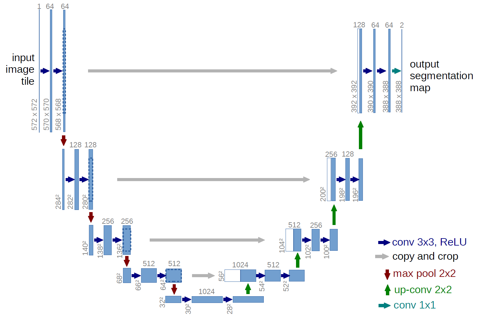
U-Net 网络是一种经典的编码器-解码器结构,因其整体结构形似大写的英文字母“U”而得名。它广泛应用于医学图像分割等领域。U-Net 的设计非常简洁:前半部分用于特征提取(编码器),后半部分用于上采样(解码器)。
编码器(Encoder)
编码器位于网络的左半部分,主要由多个下采样模块组成。每个模块包含两个 3×3 的卷积层(激活函数为 ReLU),后接一个 2×2 的最大池化(Max Pooling)层,用于特征提取和空间尺寸的减半。通过这种结构,编码器能够逐步提取图像的深层特征,同时扩大感受野。
解码器(Decoder)
解码器位于网络的右半部分,主要由上采样模块组成。每个模块包含一个 2×2 的反卷积层(上采样卷积层),用于将特征图的空间尺寸恢复到与编码器对应层相同的大小。随后,解码器通过特征拼接(concatenation)将上采样后的特征图与编码器中对应层的特征图进行通道级拼接,最后通过两个 3×3 的卷积层(激活函数为 ReLU)进一步融合特征。这种结构能够有效地结合深层特征和浅层特征,兼顾全局语义信息和局部细节。
特征融合方式
与 FCN 网络通过特征图对应像素值的相加来融合特征不同,U-Net 采用通道级拼接的方式。这种方式可以形成更厚的特征图,从而保留更多的细节信息,但也增加了显存的消耗。
U-Net 的优点
- 多尺度特征融合:U-Net 通过拼接深层和浅层特征图,能够充分利用不同层次的特征。浅层卷积关注纹理和细节特征,而深层网络关注更高级的语义特征。这种融合方式使得模型能够更好地处理复杂的分割任务。
- 边缘特征的保留:在下采样过程中,虽然会损失一些边缘特征,但通过特征拼接,解码器能够从编码器的浅层特征中找回这些丢失的边缘信息,从而提高分割的精度。
Unet 的好处我感觉是:网络层越深得到的特征图,有着更大的视野域,浅层卷积关注纹理特征,深层网络关注本质的那种特征,所以深层浅层特征都是有格子的意义的;另外一点是通过反卷积得到的更大的尺寸的特征图的边缘,是缺少信息的,毕竟每一次下采样提炼特征的同时,也必然会损失一些边缘特征,而失去的特征并不能从上采样中找回,因此通过特征的拼接,来实现边缘特征的一个找回。
下面是其他与医学相关的数据集以及对应的提取码,有兴趣的同学可以下载下来跑一下。
| 数据集名称 | 提取码 |
| Cell dataset (dsb2018) | 5l54 |
| Liver dataset | 5l88 |
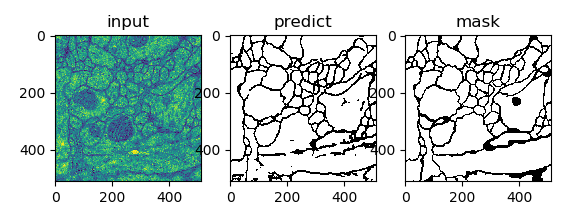
| Cell dataset (isbi) | 14rz |
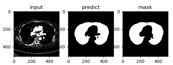
| Lung dataset | qdwo |
| Corneal Nerve dataset | ih02 |
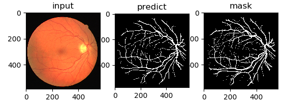
| Eye Vessels (DRIVE dataset) | f1ek |
| Esophagus and Esophagus Cancer dataset (First Affiliated Hospital of Sun Yat-sen University) | hivm |
为什么 Unet 在医疗图像分割中表现好?
大多数医疗影像语义分割任务都会首先用 Unet 作为 baseline,当然上一章节讲解的 Unet 的优点肯定是可以当作这个问题的答案,这里谈一谈医疗影像的特点
根据网友的讨论,得到的结果:
- 医疗影像语义较为简单、结构固定。因此语义信息相比自动驾驶等较为单一,因此并不需要去筛选过滤无用的信息。医疗影像的所有特征都很重要,因此低级特征和高级语义特征都很重要,所以 U 型结构的 skip connection 结构(特征拼接)更好派上用场
- 医学影像的数据较少,获取难度大,数据量可能只有几百甚至不到 100,因此如果使用大型的网络例如 DeepLabv3+ 等模型,很容易过拟合。大型网络的优点是更强的图像表述能力,而较为简单、数量少的医学影像并没有那么多的内容需要表述,因此也有人发现在小数量级中,分割的 SOTA 模型与轻量的 Unet 并没有神恶魔优势
- 医学影像往往是多模态的。比方说 ISLES 脑梗竞赛中,官方提供了 CBF,MTT,CBV 等多中模态的数据(这一点听不懂也无妨)。因此医学影像任务中,往往需要自己设计网络去提取不同的模态特征,因此轻量结构简单的 Unet 可以有更大的操作空间。
Q:过拟合与模型复杂程度有关还和什么有关呢?
模型代码
源码
import torch.nn as nn
import torch
from torch import autograd
from functools import partial
import torch.nn.functional as F
from torchvision import modelsclass DoubleConv(nn.Module):def __init__(self, in_ch, out_ch):super(DoubleConv, self).__init__()self.conv = nn.Sequential(nn.Conv2d(in_ch, out_ch, 3, _padding_=1),nn.BatchNorm2d(out_ch),nn.ReLU(_inplace_=True),nn.Conv2d(out_ch, out_ch, 3, _padding_=1),nn.BatchNorm2d(out_ch),nn.ReLU(_inplace_=True))def forward(self, input):return self.conv(input)class Unet(nn.Module):def __init__(self, in_ch, out_ch):super(Unet, self).__init__()self.conv1 = DoubleConv(in_ch, 32)self.pool1 = nn.MaxPool2d(2)self.conv2 = DoubleConv(32, 64)self.pool2 = nn.MaxPool2d(2)self.conv3 = DoubleConv(64, 128)self.pool3 = nn.MaxPool2d(2)self.conv4 = DoubleConv(128, 256)self.pool4 = nn.MaxPool2d(2)self.conv5 = DoubleConv(256, 512)self.up6 = nn.ConvTranspose2d(512, 256, 2, _stride_=2)self.conv6 = DoubleConv(512, 256)self.up7 = nn.ConvTranspose2d(256, 128, 2, _stride_=2)self.conv7 = DoubleConv(256, 128)self.up8 = nn.ConvTranspose2d(128, 64, 2, _stride_=2)self.conv8 = DoubleConv(128, 64)self.up9 = nn.ConvTranspose2d(64, 32, 2, _stride_=2)self.conv9 = DoubleConv(64, 32)self.conv10 = nn.Conv2d(32, out_ch, 1)def forward(self, x):_#print(x.shape)_c1 = self.conv1(x)p1 = self.pool1(c1)_#print(p1.shape)_c2 = self.conv2(p1)p2 = self.pool2(c2)_#print(p2.shape)_c3 = self.conv3(p2)p3 = self.pool3(c3)_#print(p3.shape)_c4 = self.conv4(p3)p4 = self.pool4(c4)_#print(p4.shape)_c5 = self.conv5(p4)up_6 = self.up6(c5)merge6 = torch.cat([up_6, c4], _dim_=1)c6 = self.conv6(merge6)up_7 = self.up7(c6)merge7 = torch.cat([up_7, c3], _dim_=1)c7 = self.conv7(merge7)up_8 = self.up8(c7)merge8 = torch.cat([up_8, c2], _dim_=1)c8 = self.conv8(merge8)up_9 = self.up9(c8)merge9 = torch.cat([up_9, c1], _dim_=1)c9 = self.conv9(merge9)c10 = self.conv10(c9)out = nn.Sigmoid()(c10)return outnonlinearity = partial(F.relu, _inplace_=True)
class DecoderBlock(nn.Module):def __init__(self, in_channels, n_filters):super(DecoderBlock, self).__init__()self.conv1 = nn.Conv2d(in_channels, in_channels // 4, 1)self.norm1 = nn.BatchNorm2d(in_channels // 4)self.relu1 = nonlinearityself.deconv2 = nn.ConvTranspose2d(in_channels // 4, in_channels // 4, 3, _stride_=2, _padding_=1, _output_padding_=1)self.norm2 = nn.BatchNorm2d(in_channels // 4)self.relu2 = nonlinearityself.conv3 = nn.Conv2d(in_channels // 4, n_filters, 1)self.norm3 = nn.BatchNorm2d(n_filters)self.relu3 = nonlinearitydef forward(self, x):x = self.conv1(x)x = self.norm1(x)x = self.relu1(x)x = self.deconv2(x)x = self.norm2(x)x = self.relu2(x)x = self.conv3(x)x = self.norm3(x)x = self.relu3(x)return xclass resnet34_unet(nn.Module):def __init__(self, num_classes=1, num_channels=3,pretrained=True):super(resnet34_unet, self).__init__()filters = [64, 128, 256, 512]resnet = models.resnet34(_pretrained_=pretrained)self.firstconv = resnet.conv1self.firstbn = resnet.bn1self.firstrelu = resnet.reluself.firstmaxpool = resnet.maxpoolself.encoder1 = resnet.layer1self.encoder2 = resnet.layer2self.encoder3 = resnet.layer3self.encoder4 = resnet.layer4self.decoder4 = DecoderBlock(512, filters[2])self.decoder3 = DecoderBlock(filters[2], filters[1])self.decoder2 = DecoderBlock(filters[1], filters[0])self.decoder1 = DecoderBlock(filters[0], filters[0])self.decoder4 = DecoderBlock(512, filters[2])self.decoder3 = DecoderBlock(filters[2], filters[1])self.decoder2 = DecoderBlock(filters[1], filters[0])self.decoder1 = DecoderBlock(filters[0], filters[0])self.finaldeconv1 = nn.ConvTranspose2d(filters[0], 32, 4, 2, 1)self.finalrelu1 = nonlinearityself.finalconv2 = nn.Conv2d(32, 32, 3, _padding_=1)self.finalrelu2 = nonlinearityself.finalconv3 = nn.Conv2d(32, num_classes, 3, _padding_=1)def forward(self, x):_# Encoder_x = self.firstconv(x)x = self.firstbn(x)x = self.firstrelu(x)x = self.firstmaxpool(x)e1 = self.encoder1(x)e2 = self.encoder2(e1)e3 = self.encoder3(e2)e4 = self.encoder4(e3)_# Center__# Decoder_d4 = self.decoder4(e4) + e3d3 = self.decoder3(d4) + e2d2 = self.decoder2(d3) + e1d1 = self.decoder1(d2)out = self.finaldeconv1(d1)out = self.finalrelu1(out)out = self.finalconv2(out)out = self.finalrelu2(out)out = self.finalconv3(out)return nn.Sigmoid()(out)
模型实现
import torch
import torch.nn as nn
import torch.nn.functional as Fclass double_conv2d_bn(nn.Module):def __init__(self,in_channels,out_channels,kernel_size=3,strides=1,padding=1):super(double_conv2d_bn,self).__init__()self.conv1 = nn.Conv2d(in_channels,out_channels,kernel_size=kernel_size,stride = strides,padding=padding,bias=True)self.conv2 = nn.Conv2d(out_channels,out_channels,kernel_size = kernel_size,stride = strides,padding=padding,bias=True)self.bn1 = nn.BatchNorm2d(out_channels)self.bn2 = nn.BatchNorm2d(out_channels)def forward(self,x):out = F.relu(self.bn1(self.conv1(x)))out = F.relu(self.bn2(self.conv2(out)))return outclass deconv2d_bn(nn.Module):def __init__(self,in_channels,out_channels,kernel_size=2,strides=2):super(deconv2d_bn,self).__init__()self.conv1 = nn.ConvTranspose2d(in_channels,out_channels,kernel_size = kernel_size,stride = strides,bias=True)self.bn1 = nn.BatchNorm2d(out_channels)def forward(self,x):out = F.relu(self.bn1(self.conv1(x)))return outclass Unet(nn.Module):def __init__(self):super(Unet,self).__init__()self.layer1_conv = double_conv2d_bn(1,8)self.layer2_conv = double_conv2d_bn(8,16)self.layer3_conv = double_conv2d_bn(16,32)self.layer4_conv = double_conv2d_bn(32,64)self.layer5_conv = double_conv2d_bn(64,128)self.layer6_conv = double_conv2d_bn(128,64)self.layer7_conv = double_conv2d_bn(64,32)self.layer8_conv = double_conv2d_bn(32,16)self.layer9_conv = double_conv2d_bn(16,8)self.layer10_conv = nn.Conv2d(8,1,kernel_size=3,stride=1,padding=1,bias=True)self.deconv1 = deconv2d_bn(128,64)self.deconv2 = deconv2d_bn(64,32)self.deconv3 = deconv2d_bn(32,16)self.deconv4 = deconv2d_bn(16,8)self.sigmoid = nn.Sigmoid()def forward(self,x):conv1 = self.layer1_conv(x)pool1 = F.max_pool2d(conv1,2)conv2 = self.layer2_conv(pool1)pool2 = F.max_pool2d(conv2,2)conv3 = self.layer3_conv(pool2)pool3 = F.max_pool2d(conv3,2)conv4 = self.layer4_conv(pool3)pool4 = F.max_pool2d(conv4,2)conv5 = self.layer5_conv(pool4)convt1 = self.deconv1(conv5)concat1 = torch.cat([convt1,conv4],dim=1)conv6 = self.layer6_conv(concat1)convt2 = self.deconv2(conv6)concat2 = torch.cat([convt2,conv3],dim=1)conv7 = self.layer7_conv(concat2)convt3 = self.deconv3(conv7)concat3 = torch.cat([convt3,conv2],dim=1)conv8 = self.layer8_conv(concat3)convt4 = self.deconv4(conv8)concat4 = torch.cat([convt4,conv1],dim=1)conv9 = self.layer9_conv(concat4)outp = self.layer10_conv(conv9)outp = self.sigmoid(outp)return outpmodel = Unet()
inp = torch.rand(10,1,224,224)
outp = model(inp)
print(outp.shape)
==> torch.Size([10, 1, 224, 224])
实例分割(Instance Segmentation)
定义
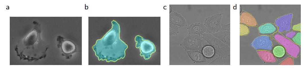
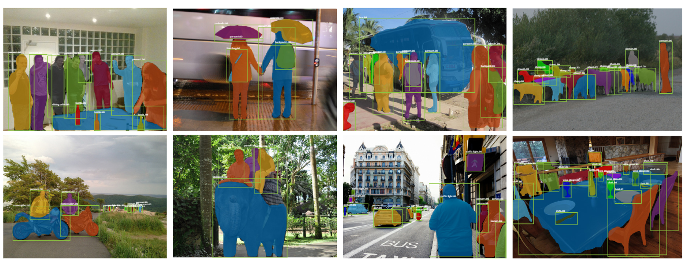
实例分割是目标检测和语义分割的结合,旨在精确识别图像中的每个目标对象,并区分同一类别中的不同实例。例如,在一张包含多个人的图像中,实例分割不仅需要识别出“人”这一类别,还需要将每个人单独区分开来,为每个人生成独立的分割掩码(Mask)。
实例分割通过融合目标检测和语义分割的结果来实现这一目标。具体而言,它利用目标检测提供的目标类别和位置信息(如边界框和置信度),从语义分割的结果中提取出对应目标的像素级掩码。简而言之,实例分割的任务是将同一类别中的具体对象(即实例)分别分割出来。
举个例子,近年来,随着自动驾驶等领域的快速发展,实例分割任务受到了广泛关注。自动驾驶场景中,精确区分和分割道路上的行人、车辆等目标对于环境感知和决策至关重要。此外,一些实例分割任务还会输出检测结果(如边界框),以提供更全面的目标描述。
对实例分割、语义分割和目标检测混合任务感兴趣的读者,可以参考 CVPR 2019 的论文《Hybrid Task Cascade》(HTC),该研究提出了一种混合任务级联框架,能够同时处理这三种任务,为多任务学习提供了新的思路。
特点
- 能够精确地定位和区分同一类别的不同实例。
- 计算成本较高,因为需要对每个目标实例进行单独检测和分类。
应用
实例分割在以下领域有重要应用:
- 自动驾驶:用于检测和分割车辆、行人。
- 医学成像:用于检测组织和病理的特定边界。
- 机器人视觉:用于识别和隔离目标物体。
常见模型
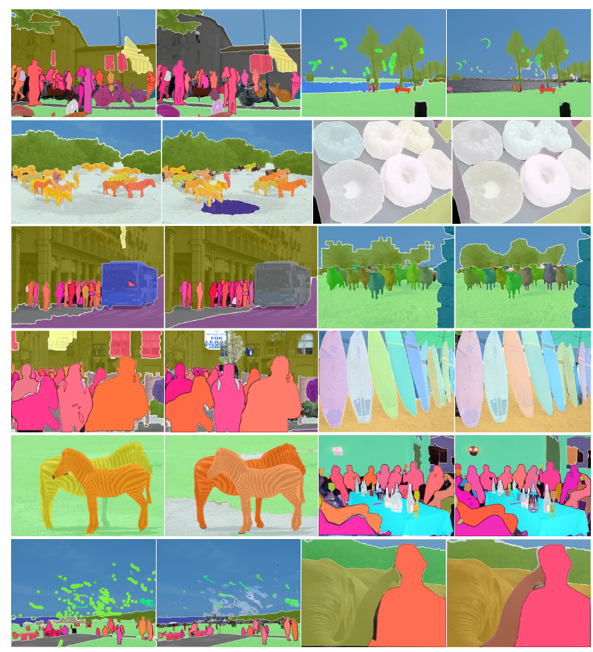
Mask R-CNN
- 优点:能够同时进行目标检测和语义分割,具有较好的性能。
- 缺点:模型参数多,训练和推理速度较慢;大目标的边缘分割较为粗糙。
提出初衷
Mask R-CNN 是 2017 年发表的文章,一作是何恺明大神,没错就是那个男人,除此之外还有 Faster R-CNN 系列的大神 Ross Girshick,可以说是强强联合。该论文也获得了 ICCV 2017 的最佳论文奖(Marr Prize)。并且该网络提出后,又霸榜了 MS COCO 的各项任务,包括目标检测、实例分割以及人体关键点检测任务。Mask R-CNN 的结构很简洁而且很灵活效果又很好(仅仅是在 Faster R-CNN 的基础上根据需求加入一些新的分支)。
Mask R-CNN 的提出初衷是为了实现高效且精确的实例分割任务,同时继承 Faster R-CNN 在目标检测方面的优势。具体而言,Mask R-CNN 的核心动机是将目标检测与语义分割相结合,既能检测图像中的目标并定位其边界框,又能为每个目标生成精确的像素级分割掩码。此外,Mask R-CNN 通过引入 RoI Align 技术,解决了 Faster R-CNN 中 RoI Pooling 导致的特征图与原始图像区域对齐不精确的问题,显著提高了分割掩码的精度。Mask R-CNN 在 Faster R-CNN 的基础上增加了全卷积网络(FCN)分支,用于预测每个感兴趣区域(RoI)的分割掩码,这种设计不仅简单高效,且只增加了较小的计算开销。
它还具备良好的多任务扩展性,能够轻松扩展到其他任务(如人体关键点检测),成为一种通用的视觉框架。通过为每个类别预测独立的二元掩码,Mask R-CNN 能够更好地提取目标的空间布局信息,从而生成更精确的分割掩码,并在 COCO 等数据集上取得了显著优于当时其他模型的性能。总之,Mask R-CNN 的提出填补了目标检测和语义分割之间的空白,提供了一种高精度、高效率的实例分割解决方案。
Mask R-CNN 的提出初衷是为了实现高效且精确的实例分割任务,同时继承 Faster R-CNN 在目标检测方面的优势。具体动机和背景如下:
- 结合目标检测与语义分割
在 Mask R-CNN 提出之前,目标检测(如 Faster R-CNN)和语义分割(如 FCN)是两个独立的领域。Mask R-CNN 的核心动机是将两者结合起来,既能够检测图像中的目标并定位其边界框,还能为每个目标生成精确的像素级分割掩码。 - 解决像素级对齐问题
Faster R-CNN 在处理像素级任务时存在局限性,尤其是其 RoI Pooling 操作会导致特征图与原始图像区域的对齐不精确。Mask R-CNN 通过引入 RoI Align 技术,解决了这一问题,显著提高了分割掩码的精度。 - 简单高效的架构设计
Mask R-CNN 在 Faster R-CNN 的基础上,增加了一个全卷积网络(FCN)分支,用于预测每个感兴趣区域(RoI)的分割掩码。这种设计不仅简单高效,而且只增加了较小的计算开销。 - 多任务学习的扩展性
Mask R-CNN 不仅适用于实例分割,还可以轻松扩展到其他任务,如人体关键点检测。这种多任务扩展性使其成为一种通用的视觉框架。 - 提升实例分割精度
通过为每个类别预测独立的二元掩码,Mask R-CNN 能够更好地提取目标的空间布局信息,从而生成更精确的分割掩码。这一改进使其在 COCO 等数据集上取得了显著优于当时其他模型的性能。
网络结构
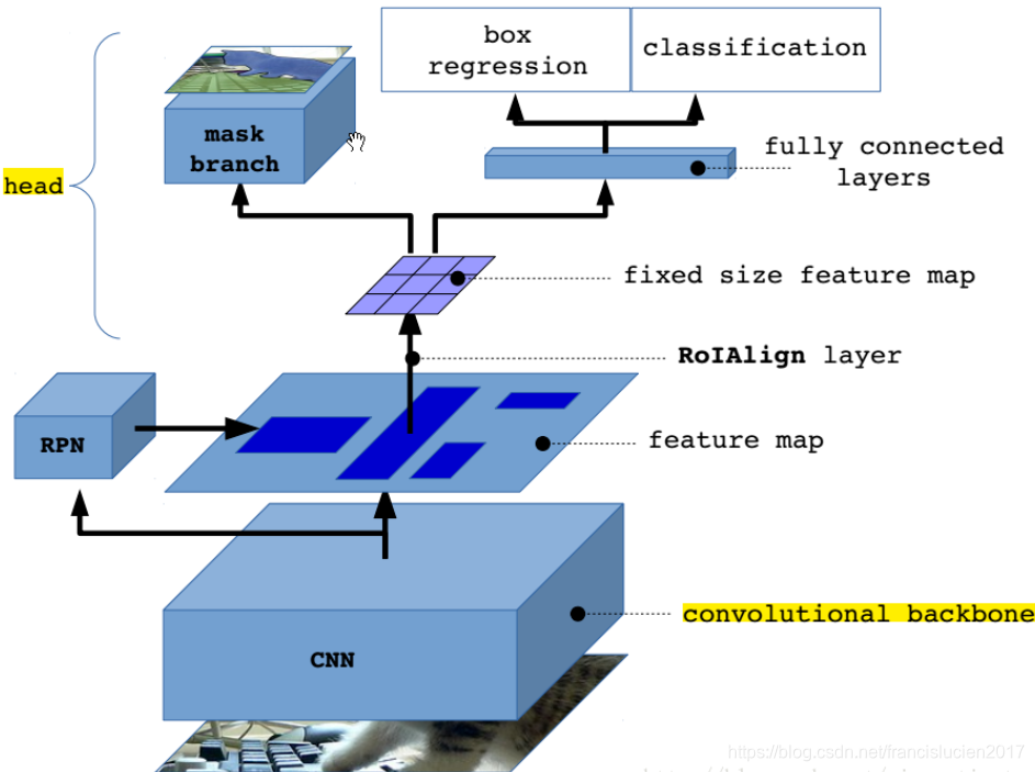
Mask R-CNN 的结构也很简单,就是在通过 RoIAlign(在原 Faster R-CNN 中是 RoIPool)得到的 RoI 基础上并行添加一个 Mask 分支(小型的 FCN)。见下图,之前 Faster R-CNN 是在 RoI 基础上接上一个 Fast R-CNN 检测头,即图中 class, box 分支,现在又并行了一个 Mask 分支。
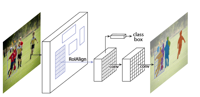
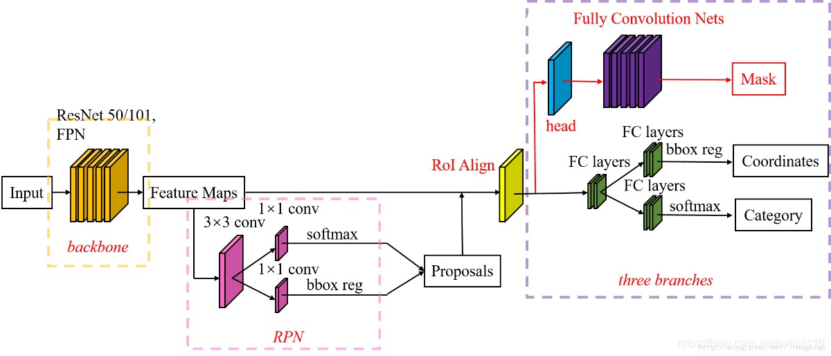
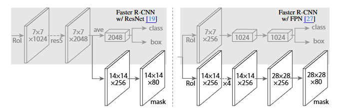
注意带和不带 FPN 结构的 Mask R-CNN 在 Mask 分支上略有不同,对于带有 FPN 结构的 Mask R-CNN 它的 class、box 分支和 Mask 分支并不是共用一个 RoIAlign。在训练过程中,对于 class, box 分支 RoIAlign 将 RPN(Region Proposal Network)得到的 Proposals 池化到 7x7 大小,而对于 Mask 分支 RoIAlign 将 Proposals 池化到 14x14 大小。
Q:Mask R-CNN 中的 RoI Align 技术是如何解决 Faster R-CNN 中 RoI Pooling 导致的特征图与原始图像区域对齐不精确的问题的呢?
模型代码
"""
Model definitions"""
from torch.autograd import Variable
import torch.nn as nn
import torch.nn.functional as F
import torch
import numpy as np
import mathfrom model.resnet import resnet50
from model.rpn import RPN
#from model.lib.roi_align.roi_align.roi_align import RoIAlign
from model.lib.roi_align.roi_align.crop_and_resize import CropAndResize
from model.lib.bbox.generate_anchors import generate_pyramid_anchors
from model.lib.bbox.nms import torch_nms as nmsdef log2_graph(x):"""Implementatin of Log2. pytorch doesn't have a native implemenation."""return torch.div(torch.log(x), math.log(2.))def ROIAlign(feature_maps, rois, config, pool_size, mode='bilinear'):"""Implements ROI Align on the features.Params:- pool_shape: [height, width] of the output pooled regions. Usually [7, 7]- image_shape: [height, width, chanells]. Shape of input image in pixelsInputs:- boxes: [batch, num_boxes, (x1, y1, x2, y2)] in normalizedcoordinates. Possibly padded with zeros if not enoughboxes to fill the array.- Feature maps: List of feature maps from different levels of the pyramid.Each is [batch, channels, height, width]Output:Pooled regions in the shape: [batch, num_boxes, height, width, channels].The width and height are those specific in the pool_shape in the layerconstructor.""""""[  x2-x1             x1 + x2 - W + 1  ][  -----      0      ---------------  ][  W - 1                  W - 1       ][                                     ][           y2-y1    y1 + y2 - H + 1  ][    0      -----    ---------------  ][           H - 1         H - 1      ]"""#feature_maps= [P2, P3, P4, P5]rois = rois.detach()crop_resize = CropAndResize(pool_size, pool_size, 0)roi_number = rois.size()[1]pooled = rois.data.new(config.IMAGES_PER_GPU*rois.size(1), 256, pool_size, pool_size).zero_()rois = rois.view(config.IMAGES_PER_GPU*rois.size(1),4)# Loop through levels and apply ROI pooling to each. P2 to P5.x_1 = rois[:, 0]y_1 = rois[:, 1]x_2 = rois[:, 2]y_2 = rois[:, 3]roi_level = log2_graph(torch.div(torch.sqrt((y_2 - y_1) * (x_2 - x_1)), 224.0))roi_level = torch.clamp(torch.clamp(torch.add(torch.round(roi_level), 4), min=2), max=5)# P2 is 256x256, P3 is 128x128, P4 is 64x64, P5 is 32x32# P2 is 4, P3 is 8, P4 is 16, P5 is 32for i, level in enumerate(range(2, 6)):scaling_ratio = 2levelheight = float(config.IMAGE_MAX_DIM)/ scaling_ratiowidth = float(config.IMAGE_MAX_DIM) / scaling_ratioixx = torch.eq(roi_level, level)box_indices = ixx.view(-1).int() * 0ix = torch.unsqueeze(ixx, 1)level_boxes = torch.masked_select(rois, ix)if level_boxes.size()[0] == 0:continuelevel_boxes = level_boxes.view(-1, 4)crops = crop_resize(feature_maps[i], torch.div(level_boxes, float(config.IMAGE_MAX_DIM))[:, [1, 0, 3, 2]], box_indices)indices_pooled = ixx.nonzero()[:, 0]pooled[indices_pooled.data, :, :, :] = crops.datapooled = pooled.view(config.IMAGES_PER_GPU, roi_number,256, pool_size, pool_size)pooled = Variable(pooled).cuda()return pooled# ---------------------------------------------------------------
# Headsclass MaskHead(nn.Module):def __init__(self, config):super(MaskHead, self).__init__()self.config = configself.num_classes = config.NUM_CLASSES#self.crop_size = config.mask_crop_size#self.roi_align = RoIAlign(self.crop_size, self.crop_size)self.conv1 = nn.Conv2d(256, 256, kernel_size=3, padding=1, stride=1)self.bn1 = nn.BatchNorm2d(256)self.conv2 = nn.Conv2d(256, 256, kernel_size=3, padding=1, stride=1)self.bn2 = nn.BatchNorm2d(256)self.conv3 = nn.Conv2d(256, 256, kernel_size=3, padding=1, stride=1)self.bn3 = nn.BatchNorm2d(256)self.conv4 = nn.Conv2d(256, 256, kernel_size=3, padding=1, stride=1)self.bn4 = nn.BatchNorm2d(256)self.deconv = nn.ConvTranspose2d(256, 256, kernel_size=4, padding=1, stride=2, bias=False)self.mask = nn.Conv2d(256, self.num_classes, kernel_size=1, padding=0, stride=1)def forward(self, x, rpn_rois):#x = self.roi_align(x, rpn_rois)x = ROIAlign(x, rpn_rois, self.config, self.config.MASK_POOL_SIZE)roi_number = x.size()[1]# merge batch and roi number togetherx = x.view(self.config.IMAGES_PER_GPU * roi_number,256, self.config.MASK_POOL_SIZE,self.config.MASK_POOL_SIZE)x = F.relu(self.bn1(self.conv1(x)), inplace=True)x = F.relu(self.bn2(self.conv2(x)), inplace=True)x = F.relu(self.bn3(self.conv3(x)), inplace=True)x = F.relu(self.bn4(self.conv4(x)), inplace=True)x = self.deconv(x)rcnn_mask_logits = self.mask(x)rcnn_mask_logits = rcnn_mask_logits.view(self.config.IMAGES_PER_GPU,roi_number,self.config.NUM_CLASSES,self.config.MASK_POOL_SIZE * 2,self.config.MASK_POOL_SIZE * 2)return rcnn_mask_logitsclass RCNNHead(nn.Module):def __init__(self, config):super(RCNNHead, self).__init__()self.config = configself.num_classes = config.NUM_CLASSES#self.crop_size = config.rcnn_crop_size#self.roi_align = RoIAlign(self.crop_size, self.crop_size)self.fc1 = nn.Linear(1024, 1024)self.fc2 = nn.Linear(1024, 1024)self.class_logits = nn.Linear(1024, self.num_classes)self.bbox = nn.Linear(1024, self.num_classes * 4)self.conv1 = nn.Conv2d(256, 1024, kernel_size=self.config.POOL_SIZE, stride=1, padding=0)self.bn1 = nn.BatchNorm2d(1024, eps=0.001)def forward(self, x, rpn_rois):x = ROIAlign(x, rpn_rois, self.config, self.config.POOL_SIZE)roi_number = x.size()[1]x = x.view(self.config.IMAGES_PER_GPU * roi_number,256, self.config.POOL_SIZE,self.config.POOL_SIZE)#print(x.shape)#x = self.roi_align(x, rpn_rois, self.config, self.config.POOL_SIZE)#x = crops.view(crops.size(0), -1)x = self.bn1(self.conv1(x))x = x.permute(0, 2, 3, 1).contiguous().view(x.size(0), -1)x = F.relu(self.fc1(x), inplace=True)x = F.relu(self.fc2(x), inplace=True)#x = F.dropout(x, 0.5, training=self.training)rcnn_class_logits = self.class_logits(x)rcnn_probs = F.softmax(rcnn_class_logits, dim=-1)rcnn_bbox = self.bbox(x)rcnn_class_logits = rcnn_class_logits.view(self.config.IMAGES_PER_GPU,roi_number,rcnn_class_logits.size()[-1])rcnn_probs = rcnn_probs.view(self.config.IMAGES_PER_GPU,roi_number,rcnn_probs.size()[-1])rcnn_bbox = rcnn_bbox.view(self.config.IMAGES_PER_GPU,roi_number,self.config.NUM_CLASSES,4)return rcnn_class_logits, rcnn_probs, rcnn_bbox#
# ---------------------------------------------------------------
# Mask R-CNNclass MaskRCNN(nn.Module):"""Mask R-CNN model"""def __init__(self, config):super(MaskRCNN, self).__init__()self.config = configself.__mode = 'train'feature_channels = 128# define modules (set of layers)
#        self.feature_net = FeatureNet(cfg, 3, feature_channels)self.feature_net = resnet50().cuda()#self.rpn_head = RpnMultiHead(cfg,feature_channels)self.rpn = RPN(256, len(self.config.RPN_ANCHOR_RATIOS),self.config.RPN_ANCHOR_STRIDE)#self.rcnn_crop = CropRoi(cfg, cfg.rcnn_crop_size)self.rcnn_head = RCNNHead(config)#self.mask_crop = CropRoi(cfg, cfg.mask_crop_size)self.mask_head = MaskHead(config)self.anchors = generate_pyramid_anchors(self.config.RPN_ANCHOR_SCALES,self.config.RPN_ANCHOR_RATIOS,self.config.BACKBONE_SHAPES,self.config.BACKBONE_STRIDES,self.config.RPN_ANCHOR_STRIDE)self.anchors = self.anchors.astype(np.float32)self.proposal_count = self.config.POST_NMS_ROIS_TRAINING# FPNself.fpn_c5p5 = nn.Conv2d(512 * 4, 256, kernel_size=1, stride=1, padding=0)self.fpn_c4p4 = nn.Conv2d(256 * 4, 256, kernel_size=1, stride=1, padding=0)self.fpn_c3p3 = nn.Conv2d(128 * 4, 256, kernel_size=1, stride=1, padding=0)self.fpn_c2p2 = nn.Conv2d(64 * 4, 256, kernel_size=1, stride=1,  padding=0)self.fpn_p2 = nn.Conv2d(256, 256, kernel_size=3, stride=1, padding=1)self.fpn_p3 = nn.Conv2d(256, 256, kernel_size=3, stride=1, padding=1)self.fpn_p4 = nn.Conv2d(256, 256, kernel_size=3, stride=1, padding=1)self.fpn_p5 = nn.Conv2d(256, 256, kernel_size=3, stride=1, padding=1)self.scale_ratios = [4, 8, 16, 32]self.fpn_p6 = nn.MaxPool2d(kernel_size=1, stride=2, padding=0, ceil_mode=False)def forward(self, x):# Extract featuresC1, C2, C3, C4, C5 = self.feature_net(x)P5 = self.fpn_c5p5(C5)P4 = self.fpn_c4p4(C4) + F.upsample(P5,scale_factor=2, mode='bilinear')P3 = self.fpn_c3p3(C3) + F.upsample(P4,scale_factor=2, mode='bilinear')P2 = self.fpn_c2p2(C2) + F.upsample(P3,scale_factor=2, mode='bilinear')# Attach 3x3 conv to all P layers to get the final feature maps.# P2 is 256, P3 is 128, P4 is 64, P5 is 32P2 = self.fpn_p2(P2)P3 = self.fpn_p3(P3)P4 = self.fpn_p4(P4)P5 = self.fpn_p5(P5)# P6 is used for the 5th anchor scale in RPN. Generated by# subsampling from P5 with stride of 2.P6 = self.fpn_p6(P5)# Note that P6 is used in RPN, but not in the classifier heads.rpn_feature_maps = [P2, P3, P4, P5, P6]self.mrcnn_feature_maps = [P2, P3, P4, P5]rpn_class_logits_outputs = []rpn_class_outputs = []rpn_bbox_outputs = []# RPN proposalsfor feature in rpn_feature_maps:rpn_class_logits, rpn_probs, rpn_bbox = self.rpn(feature)rpn_class_logits_outputs.append(rpn_class_logits)rpn_class_outputs.append(rpn_probs)rpn_bbox_outputs.append(rpn_bbox)rpn_class_logits = torch.cat(rpn_class_logits_outputs, dim=1)rpn_class = torch.cat(rpn_class_outputs, dim=1)rpn_bbox = torch.cat(rpn_bbox_outputs, dim=1)rpn_proposals = self.proposal_layer(rpn_class, rpn_bbox)# RCNN proposalsrcnn_class_logits, rcnn_class, rcnn_bbox = self.rcnn_head(self.mrcnn_feature_maps, rpn_proposals)rcnn_mask_logits = self.mask_head(self.mrcnn_feature_maps, rpn_proposals)# <todo> mask nmsreturn [rpn_class_logits, rpn_class, rpn_bbox, rpn_proposals,rcnn_class_logits, rcnn_class, rcnn_bbox,rcnn_mask_logits]def proposal_layer(self, rpn_class, rpn_bbox):# handling proposalsscores = rpn_class[:, :, 1]#print(scores.shape)# Box deltas [batch, num_rois, 4]deltas_mul = Variable(torch.from_numpy(np.reshape(self.config.RPN_BBOX_STD_DEV, [1, 1, 4]).astype(np.float32))).cuda()deltas = rpn_bbox * deltas_mulpre_nms_limit = min(6000, self.anchors.shape[0])scores, ix = torch.topk(scores, pre_nms_limit, dim=-1,largest=True, sorted=True)ix = torch.unsqueeze(ix, 2)ix = torch.cat([ix, ix, ix, ix], dim=2)deltas = torch.gather(deltas, 1, ix)_anchors = []for i in range(self.config.IMAGES_PER_GPU):anchors = Variable(torch.from_numpy(self.anchors.astype(np.float32))).cuda()_anchors.append(anchors)anchors = torch.stack(_anchors, 0)pre_nms_anchors = torch.gather(anchors, 1, ix)refined_anchors = apply_box_deltas_graph(pre_nms_anchors, deltas)# Clip to image boundaries. [batch, N, (y1, x1, y2, x2)]height, width = self.config.IMAGE_SHAPE[:2]window = np.array([0, 0, height, width]).astype(np.float32)window = Variable(torch.from_numpy(window)).cuda()refined_anchors_clipped = clip_boxes_graph(refined_anchors, window)refined_proposals = []scores = scores[:,:,None]#print(scores.data.shape)#print(refined_anchors_clipped.data.shape)for i in range(self.config.IMAGES_PER_GPU):indices = nms(torch.cat([refined_anchors_clipped.data[i], scores.data[i]], 1), 0.7)indices = indices[:self.proposal_count]indices = torch.stack([indices, indices, indices, indices], dim=1)indices = Variable(indices).cuda()proposals = torch.gather(refined_anchors_clipped[i], 0, indices)padding = self.proposal_count - proposals.size()[0]proposals = torch.cat([proposals, Variable(torch.zeros([padding, 4])).cuda()], 0)refined_proposals.append(proposals)rpn_rois = torch.stack(refined_proposals, 0)return rpn_roisdef apply_box_deltas_graph(boxes, deltas):"""Applies the given deltas to the given boxes.boxes: [N, 4] where each row is y1, x1, y2, x2deltas: [N, 4] where each row is [dy, dx, log(dh), log(dw)]"""# Convert to y, x, h, wheight = boxes[:, :, 2] - boxes[:, :, 0]width = boxes[:, :, 3] - boxes[:, :, 1]center_y = boxes[:, :, 0] + 0.5 * heightcenter_x = boxes[:, :, 1] + 0.5 * width# Apply deltascenter_y += deltas[:, :, 0] * heightcenter_x += deltas[:, :, 1] * widthheight *= torch.exp(deltas[:, :, 2])width *= torch.exp(deltas[:, :, 3])# Convert back to y1, x1, y2, x2y1 = center_y - 0.5 * heightx1 = center_x - 0.5 * widthy2 = y1 + heightx2 = x1 + widthresult = [y1, x1, y2, x2]return resultdef clip_boxes_graph(boxes, window):"""boxes: [N, 4] each row is y1, x1, y2, x2window: [4] in the form y1, x1, y2, x2"""# Split cornerswy1, wx1, wy2, wx2 = windowy1, x1, y2, x2 = boxes# Clipy1 = torch.max(torch.min(y1, wy2), wy1)x1 = torch.max(torch.min(x1, wx2), wx1)y2 = torch.max(torch.min(y2, wy2), wy1)x2 = torch.max(torch.min(x2, wx2), wx1)clipped = torch.stack([x1, y1, x2, y2], dim=2)return clipped
全景分割(Panoptic Segmentation)
定义
全景分割是语义分割和实例分割的结合。它要求对图像中的每个像素分配一个语义标签,并识别出单独的对象实例。全景分割的目标是提供一个连贯、丰富和完整的场景分割。
-
统一处理“Things”和“Stuff”:
- Things(可数目标):如人、动物、车辆等,需要检测并区分每个实例。
- Stuff(不可数目标):如天空、草地、道路等,只需进行语义分割。
全景分割通过为每个像素分配类别和实例 ID,同时处理这两种类型的目标。
-
提供完整的场景理解:
全景分割不仅关注前景目标的分割和识别,还涵盖了背景区域的语义理解,从而生成连贯且完整的场景分割。 -
解决语义分割和实例分割的局限性:
- 语义分割无法区分同一类别中的不同实例。
- 实例分割仅关注前景目标,且分割结果可能重叠。
全景分割通过统一的格式和度量,克服了这些局限性。
特点
- 同时处理“物体”(如人、车辆)和“非物体”(如草地、天空)区域。
- 输出格式为每个像素分配一个语义标签和一个唯一的实例标识符。
应用
全景分割在以下领域有重要应用:
- 自动驾驶:提供全面的场景理解,包括车辆、行人和背景。
- 增强现实:用于构建虚拟与现实融合的场景。
- 场景解析:用于复杂场景的全面理解。
常见模型
Mask2Former
- 优点:统一框架,能够处理语义、实例和全景分割任务,高精度。
- 缺点:基于 Transformer 的架构复杂,训练难度大,资源密集型。
提出初衷
Mask2Former 的提出初衷是为了进一步改进 MaskFormer 的性能,并解决其在实例分割任务中的不足。MaskFormer 虽然在多个分割任务上取得了不错的结果,但在实例分割任务上与当时的 SOTA 模型仍有较大差距,Mask2Former 的主要动机和改进点如下:
- 引入掩码注意力(Masked Attention):Mask2Former 将交叉注意力限制在预测的掩码区域内,而不是关注整个特征图。这种局部注意力机制能够更高效地提取目标特征,同时减少计算量。
- 多尺度高分辨率特征:为了更好地处理小目标,Mask2Former 利用多尺度特征金字塔,并将不同分辨率的特征分别输入到 Transformer 解码器的不同层中。这一改进显著提升了对小目标的分割性能。
- 优化训练过程:Mask2Former 对 Transformer 解码器进行了多项优化,包括调整自注意力和交叉注意力的顺序、使查询特征(query embedding)可学习、移除 dropout 等。这些改进在不增加计算开销的情况下提升了模型性能。
- 重要性采样(Importance Sampling):Mask2Former 在计算损失时,采用随机采样的方式,仅在部分像素点上计算损失,而不是在整个图像上计算。这一策略加快了训练速度。
- 通用性与高效性:Mask2Former 的目标是提供一个通用的图像分割框架,能够同时处理语义分割、实例分割和全景分割任务。相比为每个任务设计专门的模型,Mask2Former 显著减少了研究工作量,并在多个数据集上达到了 SOTA 性能。
网络结构
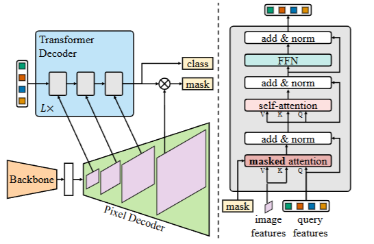
Mask2Former 是一种通用的图像分割架构,能够同时处理全景分割、实例分割和语义分割任务。其网络结构主要由以下三个核心部分组成:
1. Backbone(骨干网络)
骨干网络用于从输入图像中提取低分辨率的特征图。Mask2Former 可以使用多种流行的骨干网络,例如 ResNet 或 Swin Transformer。这些特征图将被传递到后续模块以进行进一步处理。
2. Pixel Decoder(像素解码器)
像素解码器的作用是将骨干网络提取的低分辨率特征逐步上采样到高分辨率特征图。这一模块通过多尺度特征金字塔处理不同分辨率的特征,并生成高分辨率的逐像素特征嵌入。例如,Mask2Former 使用了多尺度可变形注意力(MSDeformAttn)作为像素解码器的结构,处理 1/8、1/16、1/32 大小的特征图,并通过上采样生成 1/4 分辨率的特征图。
3. Transformer Decoder(Transformer 解码器)
Transformer 解码器是 Mask2Former 的核心模块,负责处理对象查询(object queries)并生成最终的分割掩码。Mask2Former 引入了掩码注意力(masked attention),将交叉注意力的范围限制在预测的掩码区域内,从而提取局部特征。此外,解码器还进行了多项优化:
- 掩码注意力:通过限制交叉注意力的范围,提高模型对小目标的分割性能。
- 多尺度特征利用:将不同分辨率的特征分别输入到 Transformer 解码器的不同层中,以更好地处理小目标。
- 优化训练过程:调整自注意力和交叉注意力的顺序,使查询特征可学习,并移除 dropout,从而提高计算效率。
4. 损失计算
Mask2Former 在训练时采用了一种高效的损失计算方式。它通过随机采样点计算掩码损失,而不是在整个掩码上计算损失。具体来说:
- 匹配损失(Matching Loss):在 Transformer 预测类别时,采用均匀采样计算损失。
- 最终损失(Final Loss):采用重要性采样(importance sampling),针对不同的预测结果采样不同的点计算损失。这种策略显著减少了显存占用,提高了训练效率。
Q:Mask2Former 是如何通过掩码注意力(Masked Attention)提升实例分割性能的呢?
三种分割技术的对比
语义分割、实例分割和全景分割是计算机视觉中三种重要的图像分割技术,各自有不同的任务目标、技术难点和应用场景。语义分割的目标是为图像中的每个像素分配一个类别标签,但不区分同一类别中的不同实例。它的技术难点在于需要精确的像素级分类,而对同一类别中的不同实例不进行区分。语义分割的主流方法包括 FCN、DeepLab 系列和 PSPNet,性能通常通过平均交并比(mIoU)来衡量。语义分割模型结构相对简单,适合大规模像素级分类任务,广泛应用于自动驾驶、医学影像分析和卫星图像处理等领域。
实例分割则进一步要求为图像中的每个目标实例生成独立的分割掩码,并区分同一类别中的不同实例。它的技术难点在于需要同时处理目标检测和像素级分割,尤其是在处理小目标和密集目标时,对分割精度的要求更高。实例分割的主流方法包括 Mask R-CNN、SOLO 系列和 BlendMask,性能指标通常包括掩码平均精度(mask AP)和实例分割精度。实例分割能够精确区分同一类别中的不同实例,适用于复杂场景,如自动驾驶和医学影像分析。
全景分割结合了语义分割和实例分割的优点,旨在同时处理“Things”(可数目标)和“Stuff”(不可数目标),为每个像素分配类别和实例 ID。全景分割的技术难点在于需要统一处理前景目标和背景区域,避免分割结果的重叠和遗漏。其主流方法包括 Mask2Former 和 Panoptic-DeepLab,性能通过全景质量(PQ)、分割质量(SQ)和识别质量(RQ)来衡量。全景分割提供了一种更全面的场景理解方式,适用于自动驾驶、机器人视觉和视频监控等需要完整场景理解的应用场景。
随着技术的发展,Transformer 架构逐渐被引入到这些分割任务中,显著提升了模型的多尺度特征学习能力和整体性能。语义分割、实例分割和全景分割各有其独特的优势和应用场景,但在实际应用中,全景分割因其能够提供更完整的场景理解,逐渐成为研究和应用的热点方向。
| 技术 | 方法简介 | 关注点 |
| 语义分割 | 为图像中的每个像素分配特定类别标签。 | 关注“stuff”部分 |
| 实例分割 | 在图像中检测并区分不同的物体实例。 | 关注“things”部分 |
| 全景分割 | 结合语义分割和实例分割,为每个像素分配语义标签和实例标识符。 | 同时关注“things”和“stuff”部分 |
评价指标
| 分割类型 | 评估指标 | 描述 |
| 语义分割 | 像素准确率(Pixel Accuracy) | 计算所有像素中被正确分类的比例 |
| 平均交并比(MIoU) | 衡量预测分割与真实标注之间的重叠程度,是语义分割的核心指标 | |
| Dice 系数(Dice Coefficient) | 衡量预测和真实分割的相似度,类似于 IoU | |
| 召回率(Recall)和精确率(Precision) | 分别衡量模型对正样本的召回能力和预测正样本的准确性 | |
| 实例分割 | 平均精度均值(mAP) | 通过不同交并比(IoU)阈值下的平均精度来评估模型性能,是实例分割的核心指标 |
| 平均交并比(MIoU) | 衡量预测实例与真实实例之间的重叠程度 | |
| 目标级别的精确率和召回率 | 基于实例的 IoU 判断预测实例是否正确匹配真实实例 | |
| 全景分割 | 平均交并比(mIoU) | 用于评估语义分割部分的性能 |
| 平均精度均值(mAP) | 用于评估实例分割部分的性能 | |
| 全景质量(Panoptic Quality, PQ) | 综合考虑语义分割的准确性和实例分割的完整性,是全景分割特有的评估指标 |
这些指标各有侧重点,具体选择取决于任务需求和数据集特性。
- MIoU(Mean Intersection over Union)
MIoU 是一种常用的语义分割模型评价指标,它通过计算预测结果和真实标签的交集与并集之间的比值来衡量模型性能。MIoU 的计算公式为:
M I o U = 1 N ∑ i = 1 N T P i T P i + F P i + F N i \mathrm{MIoU}=\frac1N\sum_{i=1}^N\frac{\mathrm{TP}_i}{\mathrm{TP}_i+\mathrm{FP}_i+\mathrm{FN}_i} MIoU=N1i=1∑NTPi+FPi+FNiTPi
其中 TP 表示真正例(True Positives),FP 表示假正例(False Positives),FN 表示假反例(False Negatives)。MIoU 能够综合考虑模型的像素级别预测准确度,对模型在处理不同类别、不同大小的目标时进行公平的评价。
- IoU(Intersection over Union)
IoU 指标即交并比,是语义分割中常用的标准度量。它衡量的是预测结果与真实标签之间的交集与并集之比。IoU 的计算公式为:
I o U = T P T P + F P + F N \mathrm{IoU}=\frac{\mathrm{TP}}{\mathrm{TP}+\mathrm{FP}+\mathrm{FN}} IoU=TP+FP+FNTP
- Accuracy(准确率)
A c c u r a c y = T P + T N T P + F P + F N + T N \mathrm{Accuracy}=\frac{\mathrm{TP+TN}}{\mathrm{TP+FP+FN+TN}} Accuracy=TP+FP+FN+TNTP+TN
准确率是指预测正确的样本数量占全部样本的百分比。然而,当数据类别分布不平衡时,准确率可能无法准确评价模型的好坏。因此,在语义分割任务中,准确率通常与其他指标结合使用。
- Precision(查准率,精确率)
Precision = T P T P + F P \text{Precision}=\frac{\mathrm{TP}}{\mathrm{TP}+\mathrm{FP}} Precision=TP+FPTP
查准率表示模型预测为正例的所有样本中,预测正确(真实标签为正)样本的占比。在语义分割中,查准率反映了模型对正样本的识别能力。
- Recall(查全率,召回率)
R e c a l l = T P T P + F N \mathrm{Recall}=\frac{\mathrm{TP}}{\mathrm{TP}+\mathrm{FN}} Recall=TP+FNTP
查全率表示所有真实标签为正的样本中,有多大百分比被模型预测出来。在语义分割任务中,查全率衡量了模型对正样本的覆盖程度。
- F1-Score
F1-Score 是查准率和查全率的调和平均数,用于综合评估模型的性能。它的计算公式为:
F1-Score = 2 ⋅ Precision ⋅ Recall Precision + Recall \text{F1-Score}=2\cdot\frac{\text{Precision}\cdot\text{Recall}}{\text{Precision}+\text{Recall}} F1-Score=2⋅Precision+RecallPrecision⋅Recall
F1-Score 的优点在于它综合考虑了精确度和召回率,使得模型在不平衡分类问题中的性能评估更为准确。在语义分割任务中,F1-Score 能够帮助我们了解模型在各类别上的综合表现。
- 像素准确率(Pixel Accuracy)
Pixel Accuracy = T P + T N Total Pixels \text{Pixel Accuracy}=\frac{\mathrm{TP+TN}}{\text{Total Pixels}} Pixel Accuracy=Total PixelsTP+TN
像素准确率是指模型预测正确的像素数量占总像素数量的比例。它是一个简单的指标,用于衡量模型在像素级别上的整体分类准确性。然而,像素准确率对类别不平衡的数据集不够敏感,因此通常与其他指标结合使用。
- 平均精度均值(mAP)
m A P = 1 N ∑ i = 1 N A P i \mathrm{mAP}=\frac1N\sum_{i=1}^N\mathrm{AP}_i mAP=N1i=1∑NAPi
mAP(Mean Average Precision)是一种广泛用于目标检测和实例分割任务的评价指标,也适用于全景分割。它通过计算不同类别上的平均精度(AP),并取这些值的平均值得到。mAP 综合考虑了模型的精确度(Precision)和召回率(Recall),能够更全面地评估模型在不同类别上的性能。
- 全景质量(Panoptic Quality, PQ)
全景质量(PQ)是专门为全景分割任务设计的评价指标,用于综合评估模型在处理“Things”(可数目标)和“Stuff”(不可数背景)时的性能。PQ 指标结合了分割质量(Segmentation Quality, SQ)和识别质量(Recognition Quality, RQ),并通过以下公式计算:
其中,SQ 衡量分割掩码的准确性,RQ 衡量实例识别的准确性。
PQ 指标还分为单类别 PQ 和多类别 PQ(mPQ)。在某些竞赛中,还会使用 mPQ+,即对所有图像和类别进行加权平均的 PQ,以避免因某些类别在某些图像中缺失而导致的统计偏差。
- 分割质量(Segmentation Quality, SQ)
SQ 衡量的是预测分割掩码与真实分割掩码之间的平均交并比(IoU)。具体来说,它反映了匹配成功的预测实例与真实实例之间的重叠程度。SQ 的计算公式为:S Q = ∑ ( g k , p l ) ∈ T P I o U ( g k , p l ) ∣ T P ∣ \mathrm{SQ}=\frac{\sum_{(g_k,p_l)\in\mathrm{TP}}\mathrm{IoU}(g_k,p_l)}{|\mathrm{TP}|} SQ=∣TP∣∑(gk,pl)∈TPIoU(gk,pl)
其中, g k gk gk表示真实实例, p l p_l pl 表示预测实例,TP 表示真正例(True Positives),即预测与真实实例匹配成功的对。
- 识别质量(Recognition Quality, RQ)
RQ 衡量的是模型对目标实例的识别能力,类似于目标检测中的 F1 分数。它通过平衡精确率(Precision)和召回率(Recall)来评估模型对实例的识别效果。RQ 的计算公式为:R Q = ∣ T P ∣ ∣ T P ∣ + 1 2 ∣ F P ∣ + 1 2 ∣ F P ∣ + 1 2 ∣ F N ∣ \mathrm{RQ}=\frac{|\mathrm{TP}|}{|\mathrm{TP}|+\frac12|\mathrm{FP}|+\frac12|\mathrm{FP}|+\frac12|\mathrm{FN}|} RQ=∣TP∣+21∣FP∣+21∣FP∣+21∣FN∣∣TP∣
其中,FP 表示假正例(False Positives),FN 表示假反例(False Negatives)。
- SQ:关注分割掩码的准确性,即预测掩码与真实掩码的重叠程度。
- RQ:关注实例识别的准确性,类似于目标检测中的 F1 分数。
- PQ:通过结合 SQ 和 RQ,提供了一个综合评估全景分割模型性能的指标。
项目实践
使用 AutoDL 云服务器训练模型网络
相关命令
ssh-keygen -t rsa
- 训练所需的预训练模型文件。
链接:<u>https://pan.baidu.com/s/1Ecz-l6lFcf6HmeX_pLCXZw</u>提取码: wps9 - VOC 拓展数据集:
链接:<u>https://pan.baidu.com/s/1vkk3lMheUm6IjTXznlg7Ng</u>提取码: 44mk
python predict.py --video-path video.mp4 # 检测视频文件
如何根据自己的数据构建一个目标检测或实例分割的数据集
气泡数据集,该测试数据集用于实例分割。
总结
语义分割、实例分割和全景分割是深度学习在图像分割领域的三大重要技术。语义分割专注于像素级分类,能够识别图像中不同类别的物体,但无法区分同一类别中的不同实例,因此在某些场景中需要结合实例分割来进一步划分同类别的不同实例。实例分割则专注于目标实例的区分,能够将同一类别中的不同物体单独识别出来。全景分割则结合了语义分割和实例分割的优点,能够同时提供像素级分类和实例区分,从而实现更全面的场景理解。
相关文章:
2025-06-08-深度学习网络介绍(语义分割,实例分割,目标检测)
深度学习网络介绍(语义分割,实例分割,目标检测) 前言 在开始这篇文章之前,我们得首先弄明白,什么是图像分割? 我们知道一个图像只不过是许多像素的集合。图像分割分类是对图像中属于特定类别的像素进行分类的过程,即像素级别的…...

Caliper 配置文件解析:config.yaml 和 fisco-bcos.json 附加在caliper中执行不同的合约方法
Caliper 配置文件解析:config.yaml 和 fisco-bcos.json Caliper 是一个区块链性能基准测试工具,用于评估不同区块链平台的性能。下面我将详细解释你提供的 fisco-bcos.json 文件结构,并说明它与 config.yaml 文件的关系。 fisco-bcos.json 文件解析 这个文件是针对 FISCO…...
【Ragflow】26.RagflowPlus(v0.4.0):完善解析逻辑/文档撰写模式全新升级
概述 在历经半个月的间歇性开发后,RagflowPlus再次迎来一轮升级,正式发布v0.4.0。 开源地址:https://github.com/zstar1003/ragflow-plus 更新方法 下载仓库最新代码: git clone https://github.com/zstar1003/ragflow-plus.…...
智能照明系统:具备认知能力的“光神经网络”
智能照明系统是物联网技术与传统照明深度融合的产物,其本质是通过感知环境、解析需求、自主决策的闭环控制,重构光与人、空间、环境的关系。这一系统由智能光源、多维传感器、边缘计算单元及云端管理平台构成,形成具备认知能力的“光神经网络…...

ubuntu系统 | docker+dify+ollama+deepseek搭建本地应用
1、docker 介绍与安装 docker安装:1、Ubuntu系统安装docker_ubuntu docker run-CSDN博客 docker介绍及镜像源配置:2、ubuntu系统docker介绍及镜像源和仓库配置-CSDN博客 docker常用命令:3、ubuntu系统docker常用命令-CSDN博客 docker compose安装:4、docker compose-CS…...

Docker 镜像上传到 AWS ECR:从构建到推送的全流程
一、在 EC2 实例中安装 Docker(适用于 Amazon Linux 2) 步骤 1:连接到 EC2 实例 ssh -i your-key.pem ec2-useryour-ec2-public-ip步骤 2:安装 Docker sudo yum update -y sudo amazon-linux-extras enable docker sudo yum in…...

SpringSecurity+vue通用权限系统
SpringSecurityvue通用权限系统 采用主流的技术栈实现,Mysql数据库,SpringBoot2Mybatis Plus后端,redis缓存,安全框架 SpringSecurity ,Vue3.2Element Plus实现后台管理。基于JWT技术实现前后端分离。项目开发同时采 …...

如何在Spring Boot中使用注解动态切换实现
还在用冗长的if-else或switch语句管理多个服务实现? 相信不少Spring Boot开发者都遇到过这样的场景:需要根据不同条件动态选择不同的服务实现。 如果告诉你可以完全摆脱条件判断,让Spring自动选择合适的实现——只需要一个注解,你是否感兴趣? 本文将详细介绍这种优雅的…...
短视频时长预估算法调研
weighted LR o d d s T p 1 − p ( 1 − p ) o d d s T p ( T p o d d s ∗ p ) o d d s p o d d s T o d d s odds \frac{Tp}{1-p} \newline (1-p)odds Tp \newline (Tp odds * p) odds \newline p \frac{odds}{T odds} \newline odds1−pTp(1−p)oddsTp(Tpodds…...

基于Java的离散数学题库系统设计与实现:附完整源码与论文
JAVASQL离散数学题库管理系统 一、系统概述 本系统采用Java Swing开发桌面应用,结合SQL Server数据库实现离散数学题库的高效管理。系统支持题型分类(选择题、填空题、判断题等)、难度分级、知识点关联,并提供智能组卷、在线测试…...
)
板凳-------Mysql cookbook学习 (十--2)
5.12 模式匹配中的大小写问题 mysql> use cookbook Database changed mysql> select a like A, a regexp A; ------------------------------ | a like A | a regexp A | ------------------------------ | 1 | 1 | --------------------------…...
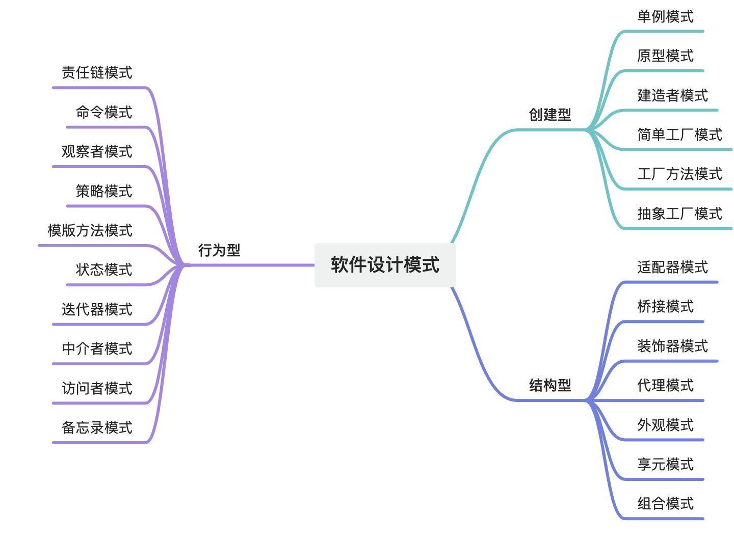
设计模式域——软件设计模式全集
摘要 软件设计模式是软件工程领域中经过验证的、可复用的解决方案,旨在解决常见的软件设计问题。它们是软件开发经验的总结,能够帮助开发人员在设计阶段快速找到合适的解决方案,提高代码的可维护性、可扩展性和可复用性。设计模式主要分为三…...
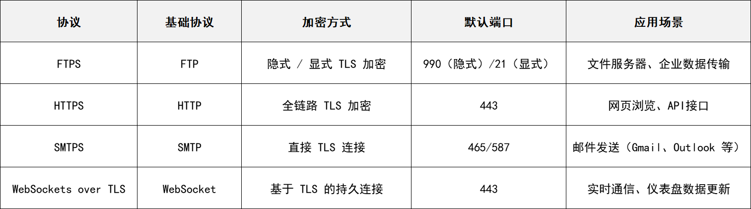
FTPS、HTTPS、SMTPS以及WebSockets over TLS的概念及其应用场景
一、什么是FTPS? FTPS,英文全称File Transfer Protocol with support for Transport Layer Security (SSL/TLS),安全文件传输协议,是一种对常用的文件传输协议(FTP)添加传输层安全(TLS)和安全套接层(SSL)加密协议支持的扩展协议。…...
--uboot系统之外设与PMIC详解)
RK3568项目(七)--uboot系统之外设与PMIC详解
目录 一、引言 二、按键 ------>2.1、按键种类 ------------>2.1.1、RESET ------------>2.1.2、UPDATE ------------>2.1.3、PWRON 部分 ------------>2.1.4、RK809 PMIC ------------>2.1.5、ADC按键 ------------>2.1.6、ADC按键驱动 ------…...
)
Three.js进阶之粒子系统(一)
一些特定模糊现象,经常使用粒子系统模拟,如火焰、爆炸等。Three.js提供了多种粒子系统,下面介绍粒子系统 一、Sprite粒子系统 使用场景:下雨、下雪、烟花 ce使用代码: var materialnew THRESS.SpriteMaterial();//…...

【仿生机器人】刀剑神域——爱丽丝苏醒计划,需求文档
仿生机器人"爱丽丝"系统架构设计需求文档 一、硬件基础 已完成头部和颈部硬件搭建 25个舵机驱动表情系统 颈部旋转功能 眼部摄像头(视觉输入) 麦克风阵列(听觉输入) 颈部发声装置(语音输出)…...

小白的进阶之路系列之十四----人工智能从初步到精通pytorch综合运用的讲解第七部分
通过示例学习PyTorch 本教程通过独立的示例介绍PyTorch的基本概念。 PyTorch的核心提供了两个主要特性: 一个n维张量,类似于numpy,但可以在gpu上运行 用于构建和训练神经网络的自动微分 我们将使用一个三阶多项式来拟合问题 y = s i n ( x ) y=sin(x) y=sin(x),作为我们的…...

JavaScript性能优化实战大纲
性能优化的核心目标 降低页面加载时间,减少内存占用,提高代码执行效率,确保流畅的用户体验。 代码层面的优化 减少全局变量使用,避免内存泄漏 // 不好的实践 var globalVar I am global;// 好的实践 (function() {var localV…...
Python 解释器安装全攻略(适用于 Linux / Windows / macOS)
目录 一、Windows安装Python解释器1.1 下载并安装Python解释1.2 测试安装是否成功1.3 设置pip的国内镜像------永久配置 二、macOS安装Python解释器三、Linux下安装Python解释器3.1 Rocky8.10/Rocky9.5安装Python解释器3.2 Ubuntu2204/Ubuntu2404安装Python解释器3.3 设置pip的…...
Java多线程从入门到精通
一、基础概念 1.1 进程与线程 进程是指运行中的程序。 比如我们使用浏览器,需要启动这个程序,操作系统会给这个程序分配一定的资源(占用内存资源)。 线程是CPU调度的基本单位,每个线程执行的都是某一个进程的代码的某…...

【芯片仿真中的X值:隐藏的陷阱与应对之道】
在芯片设计的世界里,X值(不定态)就像一个潜伏的幽灵。它可能让仿真测试顺利通过,却在芯片流片后引发灾难性后果。本文将揭开X值的本质,探讨其危害,并分享高效调试与预防的实战经验。 一、X值的本质与致…...

C++ 变量和基本类型
1、变量的声明和定义 1.1、变量声明规定了变量的类型和名字。定义初次之外,还申请存储空间,也可能会为变量赋一个初始值。 如果想声明一个变量而非定义它,就在变量名前添加关键字extern,而且不要显式地初始化变量: e…...

LeetCode第244题_最短单词距离II
LeetCode第244题:最短单词距离II 问题描述 设计一个类,接收一个单词数组 wordsDict,并实现一个方法,该方法能够计算两个不同单词在该数组中出现位置的最短距离。 你需要实现一个 WordDistance 类: WordDistance(String[] word…...

Linux 中替换文件中的某个字符串
如果你想在 Linux 中替换文件中的某个字符串,可以使用以下命令: 1. 基本替换(sed 命令) sed -i s/原字符串/新字符串/g 文件名示例:将 file.txt 中所有的 old_text 替换成 new_text sed -i s/old_text/new_text/g fi…...

python3GUI--基于PyQt5+DeepSort+YOLOv8智能人员入侵检测系统(详细图文介绍)
文章目录 一.前言二.技术介绍1.PyQt52.DeepSort3.卡尔曼滤波4.YOLOv85.SQLite36.多线程7.入侵人员检测8.ROI区域 三.核心功能1.登录注册1.登录2.注册 2.主界面1.主界面简介2.数据输入3.参数配置4.告警配置5.操作控制台6.核心内容显示区域7.检…...
5. TypeScript 类型缩小
在 TypeScript 中,类型缩小(Narrowing)是指根据特定条件将变量的类型细化为更具体的过程。它帮助开发者编写更精确、更准确的代码,确保变量在运行时只以符合其类型的方式进行处理。 一、instanceof 缩小类型 TypeScript 中的 in…...

Python_day48随机函数与广播机制
在继续讲解模块消融前,先补充几个之前没提的基础概念 尤其需要搞懂张量的维度、以及计算后的维度,这对于你未来理解复杂的网络至关重要 一、 随机张量的生成 在深度学习中经常需要随机生成一些张量,比如权重的初始化,或者计算输入…...
【QT】qtdesigner中将控件提升为自定义控件后,css设置样式不生效(已解决,图文详情)
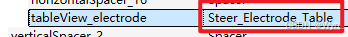
目录 0.背景 1.解决思路 2.详细代码 0.背景 实际项目中遇到的问题,描述如下: 我在qtdesigner用界面拖了一个QTableView控件,object name为【tableView_electrode】,然后【提升为】了自定义的类【Steer_Electrode_Table】&…...
【Docker 02】Docker 安装
🌈 一、各版本的平台支持情况 ⭐ 1. Server 版本 Server 版本的 Docker 就只有个命令行,没有界面。 Platformx86_64 / amd64arm64 / aarch64arm(32 - bit)s390xCentOs√√Debian√√√Fedora√√Raspbian√RHEL√SLES√Ubuntu√√√√Binaries√√√ …...

【大厂机试题+算法可视化】最长的指定瑕疵度的元音子串
题目 开头和结尾都是元音字母(aeiouAEIOU)的字符串为元音字符串,其中混杂的非元音字母数量为其瑕疵度。比如: “a” 、 “aa”是元音字符串,其瑕疵度都为0 “aiur”不是元音字符串(结尾不是元音字符) “…...