【深度学习】实验04 交叉验证
文章目录
- 交叉验证
- 划分
- 自定义划分
- K折交叉验证
- 留一交叉验证
- 留p交叉验证
- 随机排列交叉验证
- 分层K折交叉验证
- 分层随机交叉验证
- 分割
- 组 k-fold分割
- 留一组分割
- 留 P 组分割
- 随机分割
- 时间序列分割
交叉验证
# 导入相关库# 交叉验证所需函数
from sklearn.model_selection import train_test_split,cross_val_score,cross_validate
# 交叉验证所需子集划分方法
from sklearn.model_selection import KFold,LeaveOneOut,LeavePOut,ShuffleSplit
# 分层分割
from sklearn.model_selection import StratifiedKFold,StratifiedShuffleSplit
# 分组分割
from sklearn.model_selection import GroupKFold,LeaveOneGroupOut,LeavePGroupsOut,GroupShuffleSplit
# 时间序列分割
from sklearn.model_selection import TimeSeriesSplit
# 自带数据集
from sklearn import datasets
# SVM算法
from sklearn import svm
# 预处理模块
from sklearn import preprocessing
# 模型度量
from sklearn.metrics import recall_score
划分
# 加载数据集
iris = datasets.load_iris()
print('样本集大小:', iris.data.shape, iris.target.shape)
print('样本:', iris.data, iris.target)
样本集大小: (150, 4) (150,)
样本: [[5.1 3.5 1.4 0.2]
[4.9 3. 1.4 0.2]
[4.7 3.2 1.3 0.2]
[4.6 3.1 1.5 0.2]
[5. 3.6 1.4 0.2]
[5.4 3.9 1.7 0.4]
[4.6 3.4 1.4 0.3]
[5. 3.4 1.5 0.2]
[4.4 2.9 1.4 0.2]
[4.9 3.1 1.5 0.1]
[5.4 3.7 1.5 0.2]
[4.8 3.4 1.6 0.2]
[4.8 3. 1.4 0.1]
[4.3 3. 1.1 0.1]
[5.8 4. 1.2 0.2]
[5.7 4.4 1.5 0.4]
[5.4 3.9 1.3 0.4]
[5.1 3.5 1.4 0.3]
[5.7 3.8 1.7 0.3]
[5.1 3.8 1.5 0.3]
[5.4 3.4 1.7 0.2]
[5.1 3.7 1.5 0.4]
[4.6 3.6 1. 0.2]
[5.1 3.3 1.7 0.5]
[4.8 3.4 1.9 0.2]
[5. 3. 1.6 0.2]
[5. 3.4 1.6 0.4]
[5.2 3.5 1.5 0.2]
[5.2 3.4 1.4 0.2]
[4.7 3.2 1.6 0.2]
[4.8 3.1 1.6 0.2]
[5.4 3.4 1.5 0.4]
[5.2 4.1 1.5 0.1]
[5.5 4.2 1.4 0.2]
[4.9 3.1 1.5 0.1]
[5. 3.2 1.2 0.2]
[5.5 3.5 1.3 0.2]
[4.9 3.1 1.5 0.1]
[4.4 3. 1.3 0.2]
[5.1 3.4 1.5 0.2]
[5. 3.5 1.3 0.3]
[4.5 2.3 1.3 0.3]
[4.4 3.2 1.3 0.2]
[5. 3.5 1.6 0.6]
[5.1 3.8 1.9 0.4]
[4.8 3. 1.4 0.3]
[5.1 3.8 1.6 0.2]
[4.6 3.2 1.4 0.2]
[5.3 3.7 1.5 0.2]
[5. 3.3 1.4 0.2]
[7. 3.2 4.7 1.4]
[6.4 3.2 4.5 1.5]
[6.9 3.1 4.9 1.5]
[5.5 2.3 4. 1.3]
[6.5 2.8 4.6 1.5]
[5.7 2.8 4.5 1.3]
[6.3 3.3 4.7 1.6]
[4.9 2.4 3.3 1. ]
[6.6 2.9 4.6 1.3]
[5.2 2.7 3.9 1.4]
[5. 2. 3.5 1. ]
[5.9 3. 4.2 1.5]
[6. 2.2 4. 1. ]
[6.1 2.9 4.7 1.4]
[5.6 2.9 3.6 1.3]
[6.7 3.1 4.4 1.4]
[5.6 3. 4.5 1.5]
[5.8 2.7 4.1 1. ]
[6.2 2.2 4.5 1.5]
[5.6 2.5 3.9 1.1]
[5.9 3.2 4.8 1.8]
[6.1 2.8 4. 1.3]
[6.3 2.5 4.9 1.5]
[6.1 2.8 4.7 1.2]
[6.4 2.9 4.3 1.3]
[6.6 3. 4.4 1.4]
[6.8 2.8 4.8 1.4]
[6.7 3. 5. 1.7]
[6. 2.9 4.5 1.5]
[5.7 2.6 3.5 1. ]
[5.5 2.4 3.8 1.1]
[5.5 2.4 3.7 1. ]
[5.8 2.7 3.9 1.2]
[6. 2.7 5.1 1.6]
[5.4 3. 4.5 1.5]
[6. 3.4 4.5 1.6]
[6.7 3.1 4.7 1.5]
[6.3 2.3 4.4 1.3]
[5.6 3. 4.1 1.3]
[5.5 2.5 4. 1.3]
[5.5 2.6 4.4 1.2]
[6.1 3. 4.6 1.4]
[5.8 2.6 4. 1.2]
[5. 2.3 3.3 1. ]
[5.6 2.7 4.2 1.3]
[5.7 3. 4.2 1.2]
[5.7 2.9 4.2 1.3]
[6.2 2.9 4.3 1.3]
[5.1 2.5 3. 1.1]
[5.7 2.8 4.1 1.3]
[6.3 3.3 6. 2.5]
[5.8 2.7 5.1 1.9]
[7.1 3. 5.9 2.1]
[6.3 2.9 5.6 1.8]
[6.5 3. 5.8 2.2]
[7.6 3. 6.6 2.1]
[4.9 2.5 4.5 1.7]
[7.3 2.9 6.3 1.8]
[6.7 2.5 5.8 1.8]
[7.2 3.6 6.1 2.5]
[6.5 3.2 5.1 2. ]
[6.4 2.7 5.3 1.9]
[6.8 3. 5.5 2.1]
[5.7 2.5 5. 2. ]
[5.8 2.8 5.1 2.4]
[6.4 3.2 5.3 2.3]
[6.5 3. 5.5 1.8]
[7.7 3.8 6.7 2.2]
[7.7 2.6 6.9 2.3]
[6. 2.2 5. 1.5]
[6.9 3.2 5.7 2.3]
[5.6 2.8 4.9 2. ]
[7.7 2.8 6.7 2. ]
[6.3 2.7 4.9 1.8]
[6.7 3.3 5.7 2.1]
[7.2 3.2 6. 1.8]
[6.2 2.8 4.8 1.8]
[6.1 3. 4.9 1.8]
[6.4 2.8 5.6 2.1]
[7.2 3. 5.8 1.6]
[7.4 2.8 6.1 1.9]
[7.9 3.8 6.4 2. ]
[6.4 2.8 5.6 2.2]
[6.3 2.8 5.1 1.5]
[6.1 2.6 5.6 1.4]
[7.7 3. 6.1 2.3]
[6.3 3.4 5.6 2.4]
[6.4 3.1 5.5 1.8]
[6. 3. 4.8 1.8]
[6.9 3.1 5.4 2.1]
[6.7 3.1 5.6 2.4]
[6.9 3.1 5.1 2.3]
[5.8 2.7 5.1 1.9]
[6.8 3.2 5.9 2.3]
[6.7 3.3 5.7 2.5]
[6.7 3. 5.2 2.3]
[6.3 2.5 5. 1.9]
[6.5 3. 5.2 2. ]
[6.2 3.4 5.4 2.3]
[5.9 3. 5.1 1.8]] [0 0 0 0 0 0 0 0 0 0 0 0 0 0 0 0 0 0 0 0 0 0 0 0 0 0 0 0 0 0 0 0 0 0 0 0 0
0 0 0 0 0 0 0 0 0 0 0 0 0 1 1 1 1 1 1 1 1 1 1 1 1 1 1 1 1 1 1 1 1 1 1 1 1
1 1 1 1 1 1 1 1 1 1 1 1 1 1 1 1 1 1 1 1 1 1 1 1 1 1 2 2 2 2 2 2 2 2 2 2 2
2 2 2 2 2 2 2 2 2 2 2 2 2 2 2 2 2 2 2 2 2 2 2 2 2 2 2 2 2 2 2 2 2 2 2 2 2
2 2]
自定义划分
# 数据集划分
# 交叉验证划分训练集和测试集.test_size为测试集所占的比例
X_train, X_test, y_train, y_test = train_test_split(iris.data, iris.target, test_size = 0.4, random_state = 0)
print('训练集:', X_train, y_train)
print('测试集:', X_test, y_test)
训练集: [[6. 3.4 4.5 1.6]
[4.8 3.1 1.6 0.2]
[5.8 2.7 5.1 1.9]
[5.6 2.7 4.2 1.3]
[5.6 2.9 3.6 1.3]
[5.5 2.5 4. 1.3]
[6.1 3. 4.6 1.4]
[7.2 3.2 6. 1.8]
[5.3 3.7 1.5 0.2]
[4.3 3. 1.1 0.1]
[6.4 2.7 5.3 1.9]
[5.7 3. 4.2 1.2]
[5.4 3.4 1.7 0.2]
[5.7 4.4 1.5 0.4]
[6.9 3.1 4.9 1.5]
[4.6 3.1 1.5 0.2]
[5.9 3. 5.1 1.8]
[5.1 2.5 3. 1.1]
[4.6 3.4 1.4 0.3]
[6.2 2.2 4.5 1.5]
[7.2 3.6 6.1 2.5]
[5.7 2.9 4.2 1.3]
[4.8 3. 1.4 0.1]
[7.1 3. 5.9 2.1]
[6.9 3.2 5.7 2.3]
[6.5 3. 5.8 2.2]
[6.4 2.8 5.6 2.1]
[5.1 3.8 1.6 0.2]
[4.8 3.4 1.6 0.2]
[6.5 3.2 5.1 2. ]
[6.7 3.3 5.7 2.1]
[4.5 2.3 1.3 0.3]
[6.2 3.4 5.4 2.3]
[4.9 3. 1.4 0.2]
[5.7 2.5 5. 2. ]
[6.9 3.1 5.4 2.1]
[4.4 3.2 1.3 0.2]
[5. 3.6 1.4 0.2]
[7.2 3. 5.8 1.6]
[5.1 3.5 1.4 0.3]
[4.4 3. 1.3 0.2]
[5.4 3.9 1.7 0.4]
[5.5 2.3 4. 1.3]
[6.8 3.2 5.9 2.3]
[7.6 3. 6.6 2.1]
[5.1 3.5 1.4 0.2]
[4.9 3.1 1.5 0.1]
[5.2 3.4 1.4 0.2]
[5.7 2.8 4.5 1.3]
[6.6 3. 4.4 1.4]
[5. 3.2 1.2 0.2]
[5.1 3.3 1.7 0.5]
[6.4 2.9 4.3 1.3]
[5.4 3.4 1.5 0.4]
[7.7 2.6 6.9 2.3]
[4.9 2.4 3.3 1. ]
[7.9 3.8 6.4 2. ]
[6.7 3.1 4.4 1.4]
[5.2 4.1 1.5 0.1]
[6. 3. 4.8 1.8]
[5.8 4. 1.2 0.2]
[7.7 2.8 6.7 2. ]
[5.1 3.8 1.5 0.3]
[4.7 3.2 1.6 0.2]
[7.4 2.8 6.1 1.9]
[5. 3.3 1.4 0.2]
[6.3 3.4 5.6 2.4]
[5.7 2.8 4.1 1.3]
[5.8 2.7 3.9 1.2]
[5.7 2.6 3.5 1. ]
[6.4 3.2 5.3 2.3]
[6.7 3. 5.2 2.3]
[6.3 2.5 4.9 1.5]
[6.7 3. 5. 1.7]
[5. 3. 1.6 0.2]
[5.5 2.4 3.7 1. ]
[6.7 3.1 5.6 2.4]
[5.8 2.7 5.1 1.9]
[5.1 3.4 1.5 0.2]
[6.6 2.9 4.6 1.3]
[5.6 3. 4.1 1.3]
[5.9 3.2 4.8 1.8]
[6.3 2.3 4.4 1.3]
[5.5 3.5 1.3 0.2]
[5.1 3.7 1.5 0.4]
[4.9 3.1 1.5 0.1]
[6.3 2.9 5.6 1.8]
[5.8 2.7 4.1 1. ]
[7.7 3.8 6.7 2.2]
[4.6 3.2 1.4 0.2]] [1 0 2 1 1 1 1 2 0 0 2 1 0 0 1 0 2 1 0 1 2 1 0 2 2 2 2 0 0 2 2 0 2 0 2 2 0
0 2 0 0 0 1 2 2 0 0 0 1 1 0 0 1 0 2 1 2 1 0 2 0 2 0 0 2 0 2 1 1 1 2 2 1 1
0 1 2 2 0 1 1 1 1 0 0 0 2 1 2 0]
测试集: [[5.8 2.8 5.1 2.4]
[6. 2.2 4. 1. ]
[5.5 4.2 1.4 0.2]
[7.3 2.9 6.3 1.8]
[5. 3.4 1.5 0.2]
[6.3 3.3 6. 2.5]
[5. 3.5 1.3 0.3]
[6.7 3.1 4.7 1.5]
[6.8 2.8 4.8 1.4]
[6.1 2.8 4. 1.3]
[6.1 2.6 5.6 1.4]
[6.4 3.2 4.5 1.5]
[6.1 2.8 4.7 1.2]
[6.5 2.8 4.6 1.5]
[6.1 2.9 4.7 1.4]
[4.9 3.1 1.5 0.1]
[6. 2.9 4.5 1.5]
[5.5 2.6 4.4 1.2]
[4.8 3. 1.4 0.3]
[5.4 3.9 1.3 0.4]
[5.6 2.8 4.9 2. ]
[5.6 3. 4.5 1.5]
[4.8 3.4 1.9 0.2]
[4.4 2.9 1.4 0.2]
[6.2 2.8 4.8 1.8]
[4.6 3.6 1. 0.2]
[5.1 3.8 1.9 0.4]
[6.2 2.9 4.3 1.3]
[5. 2.3 3.3 1. ]
[5. 3.4 1.6 0.4]
[6.4 3.1 5.5 1.8]
[5.4 3. 4.5 1.5]
[5.2 3.5 1.5 0.2]
[6.1 3. 4.9 1.8]
[6.4 2.8 5.6 2.2]
[5.2 2.7 3.9 1.4]
[5.7 3.8 1.7 0.3]
[6. 2.7 5.1 1.6]
[5.9 3. 4.2 1.5]
[5.8 2.6 4. 1.2]
[6.8 3. 5.5 2.1]
[4.7 3.2 1.3 0.2]
[6.9 3.1 5.1 2.3]
[5. 3.5 1.6 0.6]
[5.4 3.7 1.5 0.2]
[5. 2. 3.5 1. ]
[6.5 3. 5.5 1.8]
[6.7 3.3 5.7 2.5]
[6. 2.2 5. 1.5]
[6.7 2.5 5.8 1.8]
[5.6 2.5 3.9 1.1]
[7.7 3. 6.1 2.3]
[6.3 3.3 4.7 1.6]
[5.5 2.4 3.8 1.1]
[6.3 2.7 4.9 1.8]
[6.3 2.8 5.1 1.5]
[4.9 2.5 4.5 1.7]
[6.3 2.5 5. 1.9]
[7. 3.2 4.7 1.4]
[6.5 3. 5.2 2. ]] [2 1 0 2 0 2 0 1 1 1 2 1 1 1 1 0 1 1 0 0 2 1 0 0 2 0 0 1 1 0 2 1 0 2 2 1 0
1 1 1 2 0 2 0 0 1 2 2 2 2 1 2 1 1 2 2 2 2 1 2]
# 训练模型
clf = svm.SVC(kernel = 'linear', C = 1).fit(X_train, y_train)
# 计算准确率
print('准确率:', clf.score(X_test, y_test))
准确率: 0.9666666666666667
# 如果涉及到归一化,则在测试集上也要使用训练集模型提取的归一化函数。
# 通过训练集获得归一化函数模型。(也就是先减几,再除以几的函数)。在训练集和测试集上都使用这个归一化函数
scaler = preprocessing.StandardScaler()
X_train_transformed = scaler.fit_transform(X_train)
clf = svm.SVC(kernel = 'linear', C = 1).fit(X_train_transformed, y_train)
X_test_transformed = scaler.fit_transform(X_test)
print('准确率:', clf.score(X_test_transformed, y_test))
准确率: 0.9333333333333333
# 直接调用交叉验证评估模型
clf = svm.SVC(kernel = 'linear', C = 1)
scores = cross_val_score(clf, iris.data, iris.target, cv = 5)
# 打印输出每次迭代的度量值(准确度)
print(scores)
# 获取置信区间。(也就是均值和方差)
print("Accuracy: %0.2f (+/- %0.2f)" % (scores.mean(), scores.std() * 2))
[0.96666667 1.         0.96666667 0.96666667 1.        ]
Accuracy: 0.98 (+/- 0.03)
# 多种度量结果
# precision_macro为精度,recall_macro为召回率
scoring = ['precision_macro', 'recall_macro']
scores = cross_validate(clf, iris.data, iris.target, scoring = scoring, cv = 5, return_train_score = True)
# scores类型为字典。包含训练得分,拟合次数, score-times (得分次数)
sorted(scores.keys())
print('测试结果:', scores)
测试结果: {'fit_time': array([0.00113702, 0.00095534, 0.0007391 , 0.00055671, 0.0003612 ]), 'score_time': array([0.00205898, 0.00153756, 0.00125694, 0.00080943, 0.00079727]), 'test_precision_macro': array([0.96969697, 1. , 0.96969697, 0.96969697, 1. ]), 'train_precision_macro': array([0.97674419, 0.97674419, 0.99186992, 0.98412698, 0.98333333]), 'test_recall_macro': array([0.96666667, 1. , 0.96666667, 0.96666667, 1. ]), 'train_recall_macro': array([0.975 , 0.975 , 0.99166667, 0.98333333, 0.98333333])}
K折交叉验证
# K折交叉验证
kf = KFold(n_splits = 2)
for train, test in kf.split(iris.data):print("k折划分:%s %s" % (train.shape, test.shape))break
k折划分:(75,) (75,)
留一交叉验证
#留一交叉验证
loo = LeaveOneOut()
for train, test in loo.split(iris.data):print("留一划分:%s %s" % (train.shape, test.shape))break
留一划分:(149,) (1,)
留p交叉验证
# 留p交叉验证
lpo = LeavePOut(p=2)
for train, test in loo.split(iris.data):print("留p划分:%s %s" % (train.shape, test.shape))break
留p划分:(149,) (1,)
随机排列交叉验证
# 随机排列交叉验证
ss = ShuffleSplit(n_splits=3, test_size=0.25,random_state=0)
for train_index, test_index in ss.split(iris.data):print("随机排列划分:%s %s" % (train.shape, test.shape))break
随机排列划分:(149,) (1,)
分层K折交叉验证
# 分层K折交叉验证
skf = StratifiedKFold(n_splits=3)  #各个类别的比例大致和完整数据集中相同
for train, test in skf.split(iris.data, iris.target):print("分层K折划分:%s %s" % (train.shape, test.shape))break
分层K折划分:(99,) (51,)
分层随机交叉验证
# 分层随机交叉验证
skf = StratifiedShuffleSplit(n_splits=3)  # 划分中每个类的比例和完整数据集中的相同
for train, test in skf.split(iris.data, iris.target):print("分层随机划分:%s %s" % (train.shape, test.shape))break
分层随机划分:(135,) (15,)
分割
X = [0.1, 0.2, 2.2, 2.4, 2.3, 4.55, 5.8, 8.8, 9, 10]
y = ["a", "b", "b", "b", "c", "c", "c", "d", "d", "d"]
groups = [1, 1, 1, 2, 2, 2, 3, 3, 3, 3]
组 k-fold分割
# k折分组
gkf = GroupKFold(n_splits=3)  # 训练集和测试集属于不同的组
for train, test in gkf.split(X, y, groups=groups):print("组 k-fold分割:%s %s" % (train, test))
组 k-fold分割:[0 1 2 3 4 5] [6 7 8 9]
组 k-fold分割:[0 1 2 6 7 8 9] [3 4 5]
组 k-fold分割:[3 4 5 6 7 8 9] [0 1 2]
留一组分割
# 留一分组
logo = LeaveOneGroupOut()
for train, test in logo.split(X, y, groups=groups):print("留一组分割:%s %s" % (train, test))
留一组分割:[3 4 5 6 7 8 9] [0 1 2]
留一组分割:[0 1 2 6 7 8 9] [3 4 5]
留一组分割:[0 1 2 3 4 5] [6 7 8 9]
留 P 组分割
# 留p分组
lpgo = LeavePGroupsOut(n_groups=2)
for train, test in lpgo.split(X, y, groups=groups):print("留 P 组分割:%s %s" % (train, test))
留 P 组分割:[6 7 8 9] [0 1 2 3 4 5]
留 P 组分割:[3 4 5] [0 1 2 6 7 8 9]
留 P 组分割:[0 1 2] [3 4 5 6 7 8 9]
随机分割
# 随机分组
gss = GroupShuffleSplit(n_splits=4, test_size=0.5, random_state=0)
for train, test in gss.split(X, y, groups=groups):print("随机分割:%s %s" % (train, test))
随机分割:[0 1 2] [3 4 5 6 7 8 9]
随机分割:[3 4 5] [0 1 2 6 7 8 9]
随机分割:[3 4 5] [0 1 2 6 7 8 9]
随机分割:[3 4 5] [0 1 2 6 7 8 9]
时间序列分割
# 时间序列分割
tscv = TimeSeriesSplit(n_splits=3)
TimeSeriesSplit(max_train_size=None, n_splits=3)
for train, test in tscv.split(iris.data):print("时间序列分割:%s %s" % (train, test))
时间序列分割:[ 0  1  2  3  4  5  6  7  8  9 10 11 12 13 14 15 16 17 18 19 20 21 22 2324 25 26 27 28 29 30 31 32 33 34 35 36 37 38] [39 40 41 42 43 44 45 46 47 48 49 50 51 52 53 54 55 56 57 58 59 60 61 6263 64 65 66 67 68 69 70 71 72 73 74 75]
时间序列分割:[ 0  1  2  3  4  5  6  7  8  9 10 11 12 13 14 15 16 17 18 19 20 21 22 2324 25 26 27 28 29 30 31 32 33 34 35 36 37 38 39 40 41 42 43 44 45 46 4748 49 50 51 52 53 54 55 56 57 58 59 60 61 62 63 64 65 66 67 68 69 70 7172 73 74 75] [ 76  77  78  79  80  81  82  83  84  85  86  87  88  89  90  91  92  9394  95  96  97  98  99 100 101 102 103 104 105 106 107 108 109 110 111112]
时间序列分割:[  0   1   2   3   4   5   6   7   8   9  10  11  12  13  14  15  16  1718  19  20  21  22  23  24  25  26  27  28  29  30  31  32  33  34  3536  37  38  39  40  41  42  43  44  45  46  47  48  49  50  51  52  5354  55  56  57  58  59  60  61  62  63  64  65  66  67  68  69  70  7172  73  74  75  76  77  78  79  80  81  82  83  84  85  86  87  88  8990  91  92  93  94  95  96  97  98  99 100 101 102 103 104 105 106 107108 109 110 111 112] [113 114 115 116 117 118 119 120 121 122 123 124 125 126 127 128 129 130131 132 133 134 135 136 137 138 139 140 141 142 143 144 145 146 147 148149]
相关文章:

【深度学习】实验04 交叉验证
文章目录 交叉验证划分自定义划分K折交叉验证留一交叉验证留p交叉验证随机排列交叉验证分层K折交叉验证分层随机交叉验证 分割组 k-fold分割留一组分割留 P 组分割随机分割时间序列分割 交叉验证 # 导入相关库# 交叉验证所需函数 from sklearn.model_selection import train_t…...
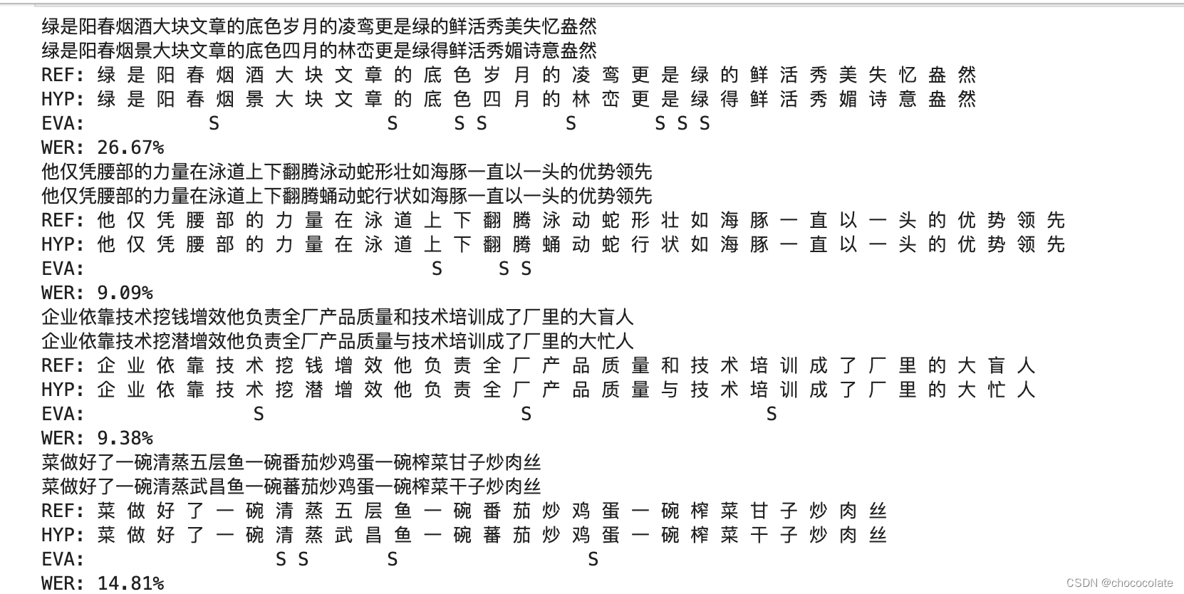
whisper语音识别部署及WER评价
1.whisper部署 详细过程可以参照:🏠 创建项目文件夹 mkdir whisper cd whisper conda创建虚拟环境 conda create -n py310 python3.10 -c conda-forge -y 安装pytorch pip install --pre torch torchvision torchaudio --extra-index-url 下载whisper p…...

java太卷了,怎么办?
忧虑: 马上就到30岁了,最近对于自己职业生涯的规划甚是焦虑。在网站论坛上,可谓是哀鸿遍野,大家纷纷叙述着自己被裁后求职的艰辛路程,这更加加深了我的忧虑,于是在各大论坛开始“求医问药”,想…...

android多屏触摸相关的详解方案-安卓framework开发手机车载车机系统开发课程
背景 直播免费视频课程地址:https://www.bilibili.com/video/BV1hN4y1R7t2/ 在做双屏相关需求开发过程中,经常会有对两个屏幕都要求可以正确触摸的场景。但是目前我们模拟器默认创建的双屏其实是没有办法进行触摸的 修改方案1 静态修改方案 使用命令…...
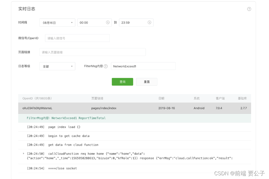
微信小程序 实时日志
目录 实时日志 背景 如何使用 如何查看日志 注意事项 实时日志 背景 为帮助小程序开发者快捷地排查小程序漏洞、定位问题,我们推出了实时日志功能。从基础库2.7.1开始,开发者可通过提供的接口打印日志,日志汇聚并实时上报到小程序后台…...
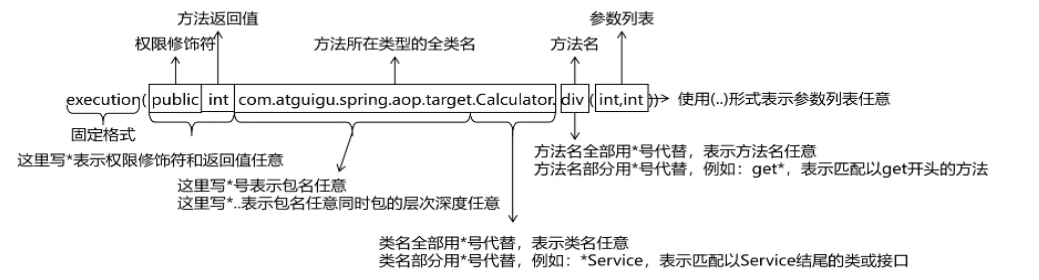
Spring AOP基于注解方式实现和细节
目录 一、Spring AOP底层技术 二、初步实现AOP编程 三、获取切点详细信息 四、 切点表达式语法 五、重用(提取)切点表达式 一、Spring AOP底层技术 SpringAop的核心在于动态代理,那么在SpringAop的底层的技术是依靠了什么技术呢&#x…...

CVPR2023论文及代码合集来啦~
以下内容由马拉AI整理汇总。 下载:点我跳转。 狂肝200小时的良心制作,529篇最新CVPR2023论文及其Code,汇总成册,制作成《CVPR 2023论文代码检索目录》,包括以下方向: 1、2D目标检测 2、视频目标检测 3、…...
基于ETLCloud的自定义规则调用第三方jar包实现繁体中文转为简体中文
背景 前面曾体验过通过零代码、可视化、拖拉拽的方式快速完成了从 MySQL 到 ClickHouse 的数据迁移,但是在实际生产环境,我们在迁移到目标库之前还需要做一些过滤和转换工作;比如,在诗词数据迁移后,发现原来 MySQL 中…...
TDesign在按钮上加入图标组件
在实际开发中 我们经常会遇到例如 添加或者查询 我们需要在按钮上加入图标的操作 TDesign自然也有预备这样的操作 首先我们打开文档看到图标 例如 我们先用某些图标 就可以点开下面的代码 可以看到 我们的图标大部分都是直接用tdesign-icons-vue 导入他的组件就可以了 而我…...
Linux 终端命令行 产品介绍
Linux命令手册内置570多个Linux 命令,内容包含 Linux 命令手册。 【软件功能】: 文件传输 bye、ftp、ftpcount、ftpshut、ftpwho、ncftp、tftp、uucico、uucp、uupick、uuto、scp备份压缩 ar、bunzip2、bzip2、bzip2recover、compress、cpio、dump、gun…...
计算机毕设 基于深度学习的植物识别算法 - cnn opencv python
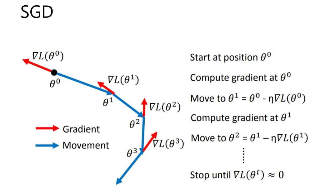
文章目录 0 前言1 课题背景2 具体实现3 数据收集和处理3 MobileNetV2网络4 损失函数softmax 交叉熵4.1 softmax函数4.2 交叉熵损失函数 5 优化器SGD6 最后 0 前言 🔥 这两年开始毕业设计和毕业答辩的要求和难度不断提升,传统的毕设题目缺少创新和亮点&a…...
【STM32】学习笔记-江科大
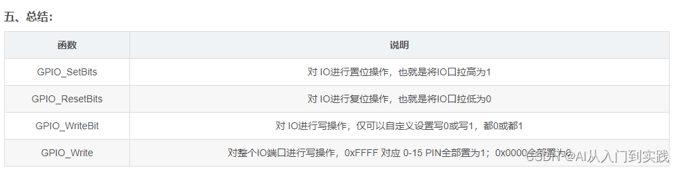
【STM32】学习笔记-江科大 1、STM32F103C8T6的GPIO口输出 2、GPIO口输出 GPIO(General Purpose Input Output)通用输入输出口可配置为8种输入输出模式引脚电平:0V~3.3V,部分引脚可容忍5V输出模式下可控制端口输出高低电平&#…...
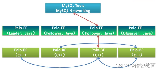
Doris架构中包含哪些技术?
Doris主要整合了Google Mesa(数据模型),Apache Impala(MPP Query Engine)和Apache ORCFile (存储格式,编码和压缩)的技术。 为什么要将这三种技术整合? Mesa可以满足我们许多存储需求的需求,但是Mesa本身不提供SQL查询引擎。 Impala是一个…...
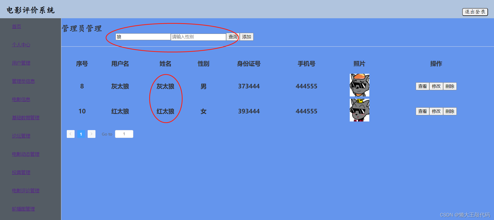
《vue3实战》通过indexOf方法实现电影评价系统的模糊查询功能
目录 前言 一、indexOf是什么?indexOf有什么作用? 含义: 作用: 二、功能实现 这段是查询过程中过滤筛选功能的代码部分: 分析: 这段是查询用户和性别功能的代码部分: 分析: 三、最终效…...
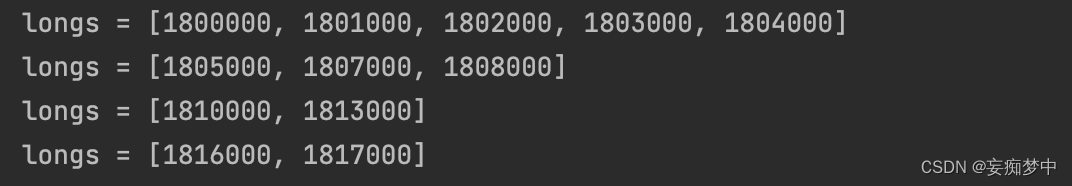
java对时间序列每x秒进行分组
问题:将一个时间序列每5秒分一组,返回嵌套的list; 原理:int除int会得到一个int(也就是损失精度) 输入:排序后的list,每几秒分组值 private static List<List<Long>> get…...

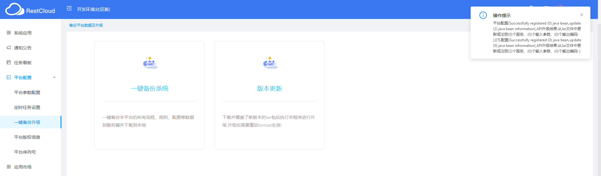
八月更新 | CI 构建计划触发机制升级、制品扫描 SBOM 分析功能上线!
点击链接了解详情 这个八月,腾讯云 CODING DevOps 对持续集成、制品管理、项目协同、平台权限等多个产品模块进行了升级改进,为用户提供更灵活便捷的使用体验。以下是 CODING 新功能速递,快来看看是否有您期待已久的功能特性: 01…...

Spring核心配置步骤-完全基于XML的配置
Spring框架的核心配置涉及多个方面,包括依赖注入(DI)、面向切面编程(AOP)等。以下是一般情况下配置Spring应用程序的核心步骤: 1. **引入Spring依赖:** 在项目的构建工具(如Maven、…...

宏基官网下载的驱动怎么安装(宏基笔记本如何安装系统)
本文为大家介绍宏基官网下载的驱动怎么安装宏基笔记本驱动(宏基笔记本如何安装系统),下面和小编一起看看详细内容吧。 宏碁笔记本怎么一键更新驱动 1. 单击“开始”,然后选择“所有程序”。 2. 单击Acer,然后单击Acer eRecovery Management。…...

基于AVR128单片机抢答器proteus仿真设计
一、系统方案 二、硬件设计 原理图如下: 三、单片机软件设计 1、首先是系统初始化 void timer0_init() //定时器初始化 { TCCR00x07; //普通模式,OC0不输出,1024分频 TCNT0f_count; //初值,定时为10ms TIFR0x01; //清中断标志…...

openGauss学习笔记-54 openGauss 高级特性-MOT
文章目录 openGauss学习笔记-54 openGauss 高级特性-MOT54.1 MOT特性及价值54.2 MOT关键技术54.3 MOT应用场景54.4 不支持的数据类型54.5 使用MOT54.6 将磁盘表转换为MOT openGauss学习笔记-54 openGauss 高级特性-MOT openGauss引入了MOT(Memory-Optimized Table&…...

如何构建高效的Azure事件驱动架构:Go SDK Messaging模块的实时消息处理指南 [特殊字符]
如何构建高效的Azure事件驱动架构:Go SDK Messaging模块的实时消息处理指南 🚀 【免费下载链接】azure-sdk-for-go This repository is for active development of the Azure SDK for Go. For consumers of the SDK we recommend visiting our public de…...

华为、华三、思科、锐捷网络设备远程登录配置
目录 一、华为Stelnet登录配置 二、华三Stelent登录配置 三、思科SSH登录配置 四、锐捷SSH登录配置 一、华为Stelnet登录配置 #查看SSH状态# [Server]dis ssh server status SSH Version : 2.0 SSH authentication timeout (Seconds) : 60 SSH authentication retries …...
基于 Transformer 架构的翻译模型实践 - 主流分词器(Tokenizer)的对比
基于 Transformer 架构的翻译模型实践 - 主流分词器(Tokenizer)的对比 flyfish 参考 https://github.com/shaoshengsong/ pytorch -transformer-en-zh-translation-demo对hello不同的分词方案可以分为单个字符【h,e,l,…...
)
uni-app项目上架前必做:手把手教你用Android Studio生成正式签名APK(从证书到发布)
uni-app项目上架全流程:从签名证书到应用商店发布的实战指南 当你完成uni-app项目的开发后,如何将代码转化为可供用户下载安装的正式APK文件?这看似简单的打包过程,实则暗藏诸多技术细节。本文将带你深入理解Android应用签名机制&…...
)
全球仅12家顶级艺术机构内部流通的Perplexity知识图谱映射表(含RIS/JSON-LD双格式导出密钥)
更多请点击: https://intelliparadigm.com 第一章:Perplexity艺术知识搜索的范式革命 传统搜索引擎依赖关键词匹配与页面权重排序,在艺术史、当代策展理论、跨媒介创作方法论等高度语境化、隐喻密集的知识领域中,常陷入“查得到却…...

Jetson Nano避坑指南:从CUDA到YOLOv5,我踩过的那些坑和最终解决方案
Jetson Nano深度排雷手册:CUDA到YOLOv5实战问题全解析 当这块信用卡大小的开发板第一次出现在我的工作台上时,我完全没预料到接下来两周会经历怎样的"技术炼狱"。从CUDA环境变量配置的幽灵报错,到PyTorch的非法指令崩溃,…...

OpenMMLab环境配置避坑指南:从CUDA 11.6到PyTorch 1.13,如何为MMRotate 0.3.4找到对的mmcv-full?
OpenMMLab精准环境配置实战:破解CUDA 11.6与PyTorch 1.13下的mmcv-full匹配困局 当你在RTX 3060显卡上尝试运行MMRotate 0.3.4时,突然发现控制台抛出ImportError: cannot import name get_dist_info from mmcv.runner——这往往是深度学习工程师与OpenMM…...

RISC-V开放架构如何重塑垂直半导体商业模式
1. 从边缘到中心:RISC-V的崛起与半导体模式的裂变最近和几位在芯片设计公司工作的老朋友聊天,话题总绕不开RISC-V。十年前,当我们还在讨论ARM和x86谁主沉浮时,RISC-V还只是学术界论文里的一个概念。如今,它已经成了行业…...
)
告别CentOS!Debian 11 + VMware 保姆级教程:搞定那些只支持国产系统的Linux客户端(以aTrust为例)
Debian 11 VMware 全栈解决方案:无缝运行国产Linux客户端软件 在开源世界的版图中,CentOS曾经是企业级Linux的代名词,但随着Red Hat战略调整和CentOS Stream的转型,许多传统解决方案正在面临前所未有的兼容性挑战。特别是在需要对…...

终极指南:如何解锁光猫全部性能?RTL960x开源方案深度解析
终极指南:如何解锁光猫全部性能?RTL960x开源方案深度解析 【免费下载链接】RTL960x Hacking & Reverse Engineering RTL960x-based xPON ONTs to suit your OLT 项目地址: https://gitcode.com/gh_mirrors/rt/RTL960x RTL960x开源光猫固件是基…...