Bert和LSTM:情绪分类中的表现
一、说明
这篇文章的目的是评估和比较 2 种深度学习算法(BERT 和 LSTM)在情感分析中进行二元分类的性能。评估将侧重于两个关键指标:准确性(衡量整体分类性能)和训练时间(评估每种算法的效率)。
二、数据
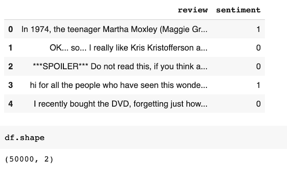
为了实现这一目标,我使用了IMDB数据集,其中包括50,000条电影评论。数据集平均分为 25,000 条正面评论和 25,000 条负面评论,使其适用于训练和测试二进制情绪分析模型。若要获取数据集,请转到以下链接:
50K电影评论的IMDB数据集
大型影评数据集
www.kaggle.com
下图显示了数据集的五行。我给积极情绪分配了 1,给消极情绪分配了 0。
三、算法
1. 长短期记忆(LSTM):它是一种循环神经网络(RNN),旨在处理顺序数据。它可以通过使用存储单元和门来捕获长期依赖关系。
2. BERT(来自变压器的双向编码器表示):它是一种预先训练的基于变压器的模型,使用自监督学习方法。利用双向上下文来理解句子中单词的含义。
-配置
对于 LSTM,模型采用文本序列以及每个序列的相应长度作为输入。它嵌入文本(嵌入维度 = 20),通过 LSTM 层(大小 = 64)处理文本,通过 ReLU 激活的全连接层传递最后一个隐藏状态,最后应用 S 形激活以生成 0 到 1 之间的单个输出值。(周期数:10,学习率:0.001,优化器:亚当)
对于BERT,我使用了DistilBertForSequenceClassification,它基于DistilBERT架构。DistilBERT是原始BERT模型的较小,蒸馏版本。它旨在具有较少数量的参数并降低计算复杂性,同时保持相似的性能水平。(周期数:3,学习率:5e-5,优化器:亚当)
四、LSTM 代码
!pip install torchtext!pip install portalocker>=2.0.0import torch
import torch.nn as nnfrom torchtext.datasets import IMDB
from torch.utils.data.dataset import random_split# Step 1: load and create the datasetstrain_dataset = IMDB(split='train')
test_dataset = IMDB(split='test')# Set random number to 123 to compare with BERT model
torch.manual_seed(123)
train_dataset, valid_dataset = random_split(list(train_dataset), [20000, 5000])## Step 2: find unique tokens (words)
import re
from collections import Counter, OrderedDicttoken_counts = Counter()def tokenizer(text):text = re.sub('<[^>]*>', '', text)emoticons = re.findall('(?::|;|=)(?:-)?(?:\)|\(|D|P)', text.lower())text = re.sub('[\W]+', ' ', text.lower()) +\' '.join(emoticons).replace('-', '')tokenized = text.split()return tokenizedfor label, line in train_dataset:tokens = tokenizer(line)token_counts.update(tokens)print('Vocab-size:', len(token_counts))## Step 3: encoding each unique token into integers
from torchtext.vocab import vocabsorted_by_freq_tuples = sorted(token_counts.items(), key=lambda x: x[1], reverse=True)
ordered_dict = OrderedDict(sorted_by_freq_tuples)vocab = vocab(ordered_dict)'''
The special tokens "<pad>" and "<unk>" are inserted into the vocabulary using vocab.insert_token("<pad>", 0) and vocab.insert_token("<unk>", 1) respectively.
The index 0 is assigned to "<pad>" token, which is typically used for padding sequences.
The index 1 is assigned to "<unk>" token, which represents unknown or out-of-vocabulary tokens.vocab.set_default_index(1) sets the default index of the vocabulary to 1, which corresponds to the "<unk>" token.
This means that if a token is not found in the vocabulary, it will be mapped to the index 1 by default.
'''vocab.insert_token("<pad>", 0)
vocab.insert_token("<unk>", 1)
vocab.set_default_index(1)print([vocab[token] for token in ['this', 'is', 'an', 'example']])'''
The IMDB class in datatext contains 1 = negative and 2 = positive
''''''
The label_pipeline lambda function takes a label value x as input.
It checks if the label value x is equal to 2 using the comparison x == 2.
If the condition is true, it returns a float value of 1.0. This implies that the label is positive.
If the condition is false (i.e., the label value is not equal to 2), it returns a float value of 0.0. This implies that the label is negative.
'''text_pipeline = lambda x: [vocab[token] for token in tokenizer(x)]
label_pipeline = lambda x: 1. if x == 2 else 0'''
This line suggests that the subsequent computations and tensors will be moved to the specified CUDA device for processing,
taking advantage of GPU acceleration if available.
'''device = torch.device("cuda:0")## Step 3-B: wrap the encode and transformation function'''
Instead of loading the whole reviews into memory which is way too expensive for the computer,
you can load a batch for manuy times which requires way less memory as compared to loading the complete data set.
Another reason that we use batch is that if we load the whole dataset at once, the deep learning algorithm(may be a neural network)
has to store errors values for all data points in the memory and this will cause a great decrease in speed of training.
With batches, the model updates the parameters(weights and bias) only after passing through the whole data set.
'''def collate_batch(batch):label_list, text_list, lengths = [], [], []for _label, _text in batch:label_list.append(label_pipeline(_label))processed_text = torch.tensor(text_pipeline(_text),dtype=torch.int64)text_list.append(processed_text)lengths.append(processed_text.size(0))## Convert lists to tensorslabel_list = torch.tensor(label_list)lengths = torch.tensor(lengths)## pads the text sequences in text_list to have the same length by adding padding tokens.padded_text_list = nn.utils.rnn.pad_sequence(text_list, batch_first=True)return padded_text_list.to(device), label_list.to(device), lengths.to(device)## Take a small batch to check if the wrapping worksfrom torch.utils.data import DataLoader
dataloader = DataLoader(train_dataset, batch_size=4, shuffle=False, collate_fn=collate_batch)
text_batch, label_batch, length_batch = next(iter(dataloader))
print(text_batch)
print(label_batch)
print(length_batch)
print(text_batch.shape)## Step 4: batching the datasetsbatch_size = 32train_dl = DataLoader(train_dataset, batch_size=batch_size,shuffle=True, collate_fn=collate_batch)
valid_dl = DataLoader(valid_dataset, batch_size=batch_size,shuffle=False, collate_fn=collate_batch)
test_dl = DataLoader(test_dataset, batch_size=batch_size,shuffle=False, collate_fn=collate_batch)print(len(list(train_dl.dataset)))
print(len(list(valid_dl.dataset)))
print(len(list(test_dl.dataset)))'''
the code defines an RNN model that takes encoded text inputs,
processes them through an embedding layer and an LSTM layer,
and produces a binary output using fully connected layers and a sigmoid activation function.
The model is initialized with specific parameters and moved to the specified device for computation.
'''class RNN(nn.Module):def __init__(self, vocab_size, embed_dim, rnn_hidden_size, fc_hidden_size):super().__init__()self.embedding = nn.Embedding(vocab_size,embed_dim,padding_idx=0)self.rnn = nn.LSTM(embed_dim, rnn_hidden_size,batch_first=True)self.fc1 = nn.Linear(rnn_hidden_size, fc_hidden_size)self.relu = nn.ReLU()self.fc2 = nn.Linear(fc_hidden_size, 1)self.sigmoid = nn.Sigmoid()def forward(self, text, lengths):out = self.embedding(text)out = nn.utils.rnn.pack_padded_sequence(out, lengths.cpu().numpy(), enforce_sorted=False, batch_first=True)out, (hidden, cell) = self.rnn(out)out = hidden[-1, :, :]out = self.fc1(out)out = self.relu(out)out = self.fc2(out)out = self.sigmoid(out)return outvocab_size = len(vocab)
embed_dim = 20
rnn_hidden_size = 64
fc_hidden_size = 64torch.manual_seed(123)
model = RNN(vocab_size, embed_dim, rnn_hidden_size, fc_hidden_size)
model = model.to(device)def train(dataloader):model.train()total_acc, total_loss = 0, 0for text_batch, label_batch, lengths in dataloader:optimizer.zero_grad()pred = model(text_batch, lengths)[:, 0]loss = loss_fn(pred, label_batch)loss.backward()optimizer.step()total_acc += ((pred>=0.5).float() == label_batch).float().sum().item()total_loss += loss.item()*label_batch.size(0)return total_acc/len(dataloader.dataset), total_loss/len(dataloader.dataset)def evaluate(dataloader):model.eval()total_acc, total_loss = 0, 0with torch.no_grad():for text_batch, label_batch, lengths in dataloader:pred = model(text_batch, lengths)[:, 0]loss = loss_fn(pred, label_batch.float())  # Convert label_batch to Floattotal_acc += ((pred >= 0.5).float() == label_batch).float().sum().item()total_loss += loss.item() * label_batch.size(0)return total_acc/len(list(dataloader.dataset)),\total_loss/len(list(dataloader.dataset))import time
start_time = time.time()loss_fn = nn.BCELoss()
optimizer = torch.optim.Adam(model.parameters(), lr=0.001)num_epochs = 10torch.manual_seed(123)for epoch in range(num_epochs):acc_train, loss_train = train(train_dl)acc_valid, loss_valid = evaluate(valid_dl)print(f'Epoch {epoch} accuracy: {acc_train:.4f} val_accuracy: {acc_valid:.4f}')print(f'Time elapsed: {(time.time() - start_time)/60:.2f} min')
print(f'Total Training Time: {(time.time() - start_time)/60:.2f} min')acc_test, _ = evaluate(test_dl)
print(f'test_accuracy: {acc_test:.4f}')"""### Test with new movie reviews of Spider-Man: Across the Spider-Verse (2023)"""def collate_single_text(text):processed_text = torch.tensor(text_pipeline(text), dtype=torch.int64)length = processed_text.size(0)padded_text = nn.utils.rnn.pad_sequence([processed_text], batch_first=True)return padded_text.to(device), lengthtext = "It is the first marvel movie to make me shed a tear. It has heart, it feels so alive with it's conveyance of emotions and feelings, it uses our nostalgia for the first movie AGAINST US it is on a completely new level of animation, there is a twist on every turn you make while watching this movie. "
padded_text, length = collate_single_text(text)
padded_text = padded_text.to(device)model.eval()  # Set the model to evaluation mode
with torch.no_grad():encoded_text = padded_text.to(device)  # Move the encoded_text tensor to the CUDA devicelengths = torch.tensor([len(encoded_text)])  # Compute the length of the text sequenceoutput = model(encoded_text, lengths)  # Pass the lengths argumentprobability = output.item()  # Obtain the predicted probabilityif probability >= 0.5:prediction = "Positive"else:prediction = "Negative"print(f"Text: {text}")
print(f"Prediction: {prediction} (Probability: {probability})")text = "This movie was very boring and garbage this is why Hollywood has zero imagination. They rewrote Spiderman as Miles Morales so that they can fit the DEI agenda which was more important than time. "
padded_text, length = collate_single_text(text)
padded_text = padded_text.to(device)model.eval()  # Set the model to evaluation mode
with torch.no_grad():encoded_text = padded_text.to(device)  # Move the encoded_text tensor to the CUDA devicelengths = torch.tensor([len(encoded_text)])  # Compute the length of the text sequenceoutput = model(encoded_text, lengths)  # Pass the lengths argumentprobability = output.item()  # Obtain the predicted probabilityif probability >= 0.5:prediction = "Positive"else:prediction = "Negative"print(f"Text: {text}")
print(f"Prediction: {prediction} (Probability: {probability})")
五、BERT代码
!pip install transformersimport gzip
import shutil
import timeimport pandas as pd
import requests
import torch
import torch.nn.functional as F
import torchtextimport transformers
from transformers import DistilBertTokenizerFast
from transformers import DistilBertForSequenceClassificationtorch.backends.cudnn.deterministic = True
RANDOM_SEED = 123
torch.manual_seed(RANDOM_SEED)
DEVICE = torch.device('cuda' if torch.cuda.is_available() else 'cpu')NUM_EPOCHS = 3path = '/content/drive/MyDrive/data/movie_data.csv'df = pd.read_csv(path)df.head()df.shapetrain_texts = df.iloc[:35000]['review'].values
train_labels = df.iloc[:35000]['sentiment'].valuesvalid_texts = df.iloc[35000:40000]['review'].values
valid_labels = df.iloc[35000:40000]['sentiment'].valuestest_texts = df.iloc[40000:]['review'].values
test_labels = df.iloc[40000:]['sentiment'].valuestokenizer = DistilBertTokenizerFast.from_pretrained('distilbert-base-uncased')train_encodings = tokenizer(list(train_texts), truncation=True, padding=True)
valid_encodings = tokenizer(list(valid_texts), truncation=True, padding=True)
test_encodings = tokenizer(list(test_texts), truncation=True, padding=True)train_encodings[0]class IMDbDataset(torch.utils.data.Dataset):def __init__(self, encodings, labels):self.encodings = encodingsself.labels = labelsdef __getitem__(self, idx):item = {key: torch.tensor(val[idx]) for key, val in self.encodings.items()}item['labels'] = torch.tensor(self.labels[idx])return itemdef __len__(self):return len(self.labels)train_dataset = IMDbDataset(train_encodings, train_labels)
valid_dataset = IMDbDataset(valid_encodings, valid_labels)
test_dataset = IMDbDataset(test_encodings, test_labels)train_loader = torch.utils.data.DataLoader(train_dataset, batch_size=16, shuffle=True)
valid_loader = torch.utils.data.DataLoader(valid_dataset, batch_size=16, shuffle=False)
test_loader = torch.utils.data.DataLoader(test_dataset, batch_size=16, shuffle=False)model = DistilBertForSequenceClassification.from_pretrained('distilbert-base-uncased')
model.to(DEVICE)
model.train()optim = torch.optim.Adam(model.parameters(), lr=5e-5)def compute_accuracy(model, data_loader, device):with torch.no_grad():correct_pred, num_examples = 0, 0for batch_idx, batch in enumerate(data_loader):### Prepare datainput_ids = batch['input_ids'].to(device)attention_mask = batch['attention_mask'].to(device)labels = batch['labels'].to(device)outputs = model(input_ids, attention_mask=attention_mask)logits = outputs['logits']predicted_labels = torch.argmax(logits, 1)num_examples += labels.size(0)correct_pred += (predicted_labels == labels).sum()return correct_pred.float()/num_examples * 100start_time = time.time()for epoch in range(NUM_EPOCHS):model.train()for batch_idx, batch in enumerate(train_loader):### Prepare datainput_ids = batch['input_ids'].to(DEVICE)attention_mask = batch['attention_mask'].to(DEVICE)labels = batch['labels'].to(DEVICE)### Forwardoutputs = model(input_ids, attention_mask=attention_mask, labels=labels)loss, logits = outputs['loss'], outputs['logits']### Backwardoptim.zero_grad()loss.backward()optim.step()### Loggingif not batch_idx % 250:print (f'Epoch: {epoch+1:04d}/{NUM_EPOCHS:04d} | 'f'Batch {batch_idx:04d}/{len(train_loader):04d} | 'f'Loss: {loss:.4f}')model.eval()with torch.set_grad_enabled(False):print(f'Training accuracy: 'f'{compute_accuracy(model, train_loader, DEVICE):.2f}%'f'\nValid accuracy: 'f'{compute_accuracy(model, valid_loader, DEVICE):.2f}%')print(f'Time elapsed: {(time.time() - start_time)/60:.2f} min')print(f'Total Training Time: {(time.time() - start_time)/60:.2f} min')
print(f'Test accuracy: {compute_accuracy(model, test_loader, DEVICE):.2f}%')
六、结果
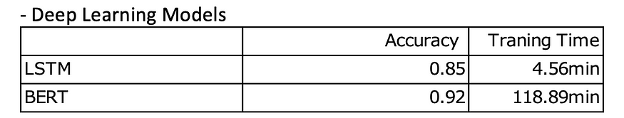
七、为什么BERT的性能优于LSTM?
BERT之所以获得高准确率,有几个原因:
1)BERT通过考虑给定单词两侧的周围单词来捕获单词的上下文含义。这种双向方法使模型能够理解语言的细微差别并有效地捕获单词之间的依赖关系。
2)BERT采用变压器架构,可有效捕获顺序数据中的长期依赖关系。转换器采用自我注意机制,使模型能够权衡句子中不同单词的重要性。这种注意力机制有助于BERT专注于相关信息,从而获得更好的表示和更高的准确性。
3)BERT在大量未标记的数据上进行预训练。这种预训练允许模型学习一般语言表示,并获得对语法、语义和世界知识的广泛理解。通过利用这些预训练的知识,BERT可以更好地适应下游任务并实现更高的准确性。
八、结论
与 LSTM 相比,BERT 确实需要更长的时间来微调,因为它的架构更复杂,参数空间更大。但同样重要的是要考虑到BERT在许多任务中的性能优于LSTM。 达门·
相关文章:
Bert和LSTM:情绪分类中的表现
一、说明 这篇文章的目的是评估和比较 2 种深度学习算法(BERT 和 LSTM)在情感分析中进行二元分类的性能。评估将侧重于两个关键指标:准确性(衡量整体分类性能)和训练时间(评估每种算法的效率)。…...

【面试经典150题】跳跃游戏
题目链接 给你一个非负整数数组 nums ,你最初位于数组的 第一个下标 。数组中的每个元素代表你在该位置可以跳跃的最大长度。 判断你是否能够到达最后一个下标,如果可以,返回 true ;否则,返回 false 。 1 < nums…...

【Rust】003-基础语法:流程控制
【Rust】003-基础语法:流程控制 文章目录 【Rust】003-基础语法:流程控制一、概述二、if 表达式1、语法格式2、多个3、获取表达式的值 三、循环1、loop:无限循环,可跳出无限循环跳出循环返回值 2、while:条件循环&…...
0829【综述】面向时空数据的区块链研究综述
摘要:时空数据包括时间和空间2个维度,常被应用于物流、供应链等领域。传统的集中式存储方式虽然具有一定的便捷性,但不能充分满足时空数据存储及查询等要求,而区块链技术采用去中心化的分布式存储机制,并通过共识协议来保证数据的安全性。研究现有区块链1.0、2.0和以Block-DAG为…...
MySQL高级篇(SQL优化、索引优化、锁机制、主从复制)
目录 0 存储引擎介绍1 SQL性能分析2 常见通用的JOIN查询 SQL执行加载顺序七种JOIN写法3 索引介绍 3.1 索引是什么3.2 索引优劣势3.3 索引分类和建索引命令语句3.4 索引结构与检索原理3.5 哪些情况适合建索引3.6 哪些情况不适合建索引4 性能分析 4.1 性能分析前提知识4.2 Expla…...
YOLOV8模型使用-检测-物体追踪
这个最新的物体检测模型,很厉害的样子,还有物体追踪的功能。 有官方的Python代码,直接上手试试就好,至于理论,有想研究在看论文了╮(╯_╰)╭ 简单介绍 YOLOv8 中可用的模型 YOLOv8 模型的每个类别中有五个模型用于检…...

springmvc:设置后端响应给前端的json数据转换成String格式
设置spring-mvc.xml: xml <?xml version"1.0" encoding"UTF-8"?> <beans xmlns"http://www.springframework.org/schema/beans"xmlns:context"http://www.springframework.org/schema/context"xmlns:xsi"http://www.w…...
Mac安装brew、mysql、redis
mac安装brew mac安装brewmac安装mysql并配置开机启动mac安装redis并配置开机启动 mac安装brew 第一步:执行. /bin/bash -c "$(curl -fsSL https://raw.githubusercontent.com/Homebrew/install/HEAD/install.sh)"第二步:输入开机密码 第三…...
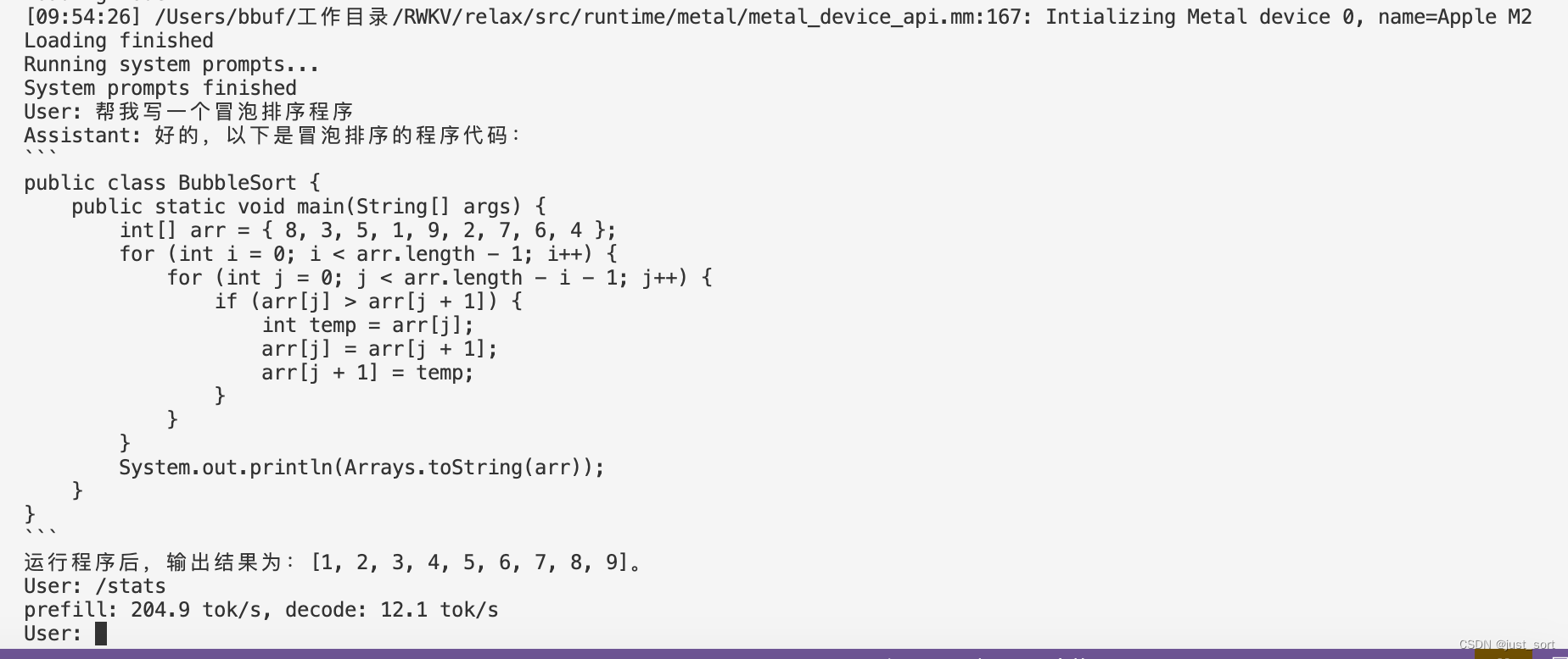
MLC-LLM 部署RWKV World系列模型实战(3B模型Mac M2解码可达26tokens/s)
0x0. 前言 我的 ChatRWKV 学习笔记和使用指南 这篇文章是学习RWKV的第一步,然后学习了一下之后决定自己应该做一些什么。所以就在RWKV社区看到了这个将RWKV World系列模型通过MLC-LLM部署在各种硬件平台的需求,然后我就开始了解MLC-LLM的编译部署流程和…...

Unity 之 参数类型之值类型参数的用法
文章目录 基本数据类型结构体结构体的进一步补充 总结: 当谈论值类型参数时,我们可以从基本数据类型和结构体两个方面详细解释。值类型参数指的是以值的形式传递给函数或方法的数据,而不是引用。 基本数据类型 基本数据类型的值类型参数&…...
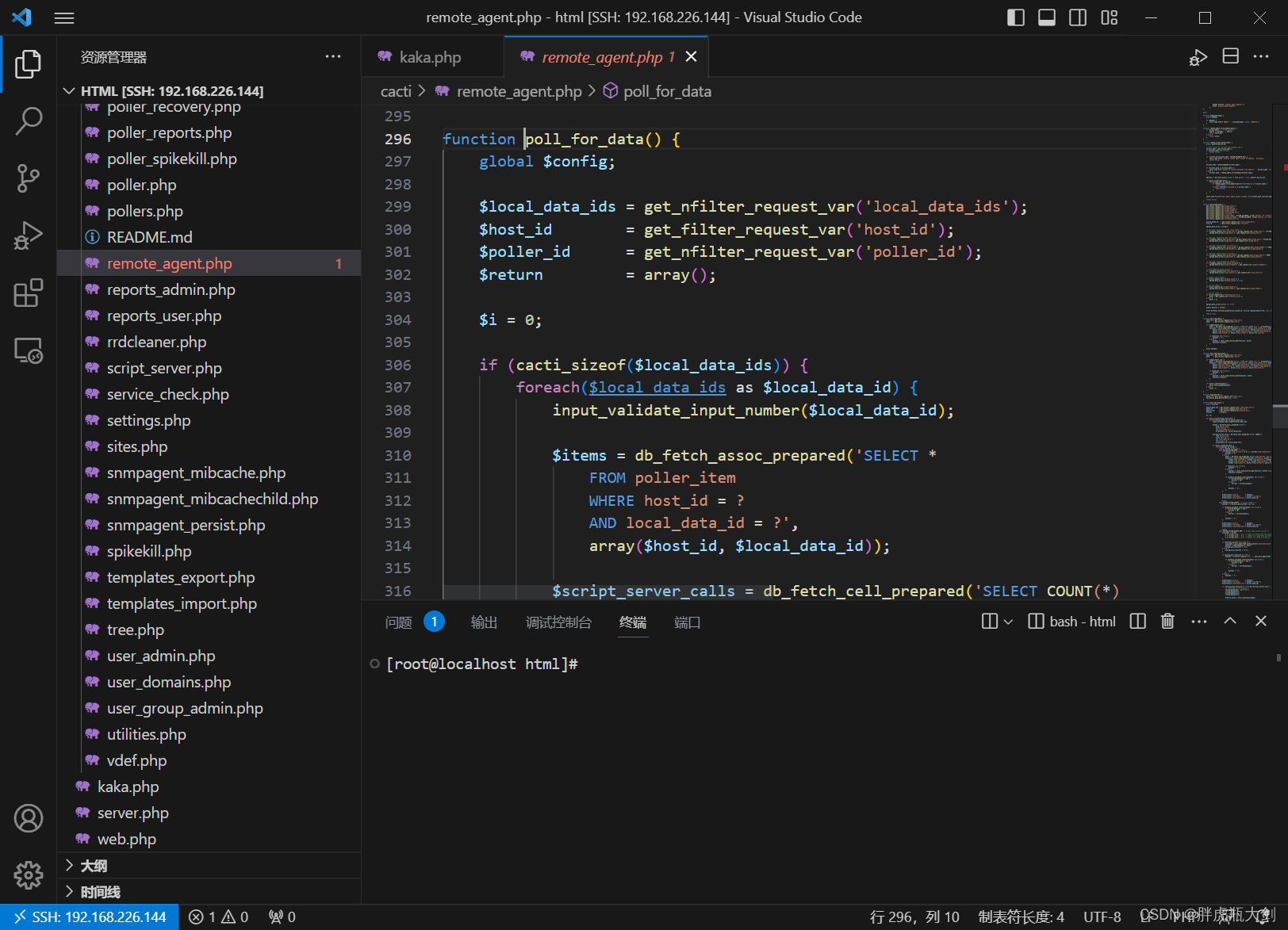
VScode远程连接主机
一、前期准备 1、Windows安装VSCode; 2、在VSCode中安装PHP Debug插件; 3、安装好Docker 4、在容器中安装Xdebug ①写一个展现phpinfo的php文件 <?php phpinfo(); ?>②在浏览器上打开该文件 ③复制所有信息丢到Xdebug: Installation instr…...
【iOS】属性关键字
文章目录 前言一、深拷贝与浅拷贝1、OC的拷贝方式有哪些2. OC对象实现的copy和mutableCopy分别为浅拷贝还是深拷贝?3. 自定义对象实现的copy和mutableCopy分别为浅拷贝还是深拷贝?4. 判断当前的深拷贝的类型?(区别是单层深拷贝还是完全深拷贝…...
【计算机基础】Git从安装到使用,详细每一步!扩展Github\Gitlab
📢:如果你也对机器人、人工智能感兴趣,看来我们志同道合✨ 📢:不妨浏览一下我的博客主页【https://blog.csdn.net/weixin_51244852】 📢:文章若有幸对你有帮助,可点赞 👍…...
深入了解Docker镜像操作
Docker是一种流行的容器化平台,它允许开发者将应用程序及其依赖项打包成容器,以便在不同环境中轻松部署和运行。在Docker中,镜像是构建容器的基础,有些家人们可能在服务器上对docker镜像的操作命令不是很熟悉,本文将深…...

嵌入式开发-单片机学习介绍
一、单片机入门篇 单片机的定义和历史 单片机是一种集成了微处理器、存储器、输入输出接口和其他功能于一体的微型计算机,具有高度的集成性和便携性。单片机的历史可以追溯到20世纪70年代,随着微电子技术的不断发展,单片机逐渐成为了工业控…...
5、Spring之Bean生命周期源码解析(销毁)
Bean的销毁过程 Bean销毁是发送在Spring容器关闭过程中的。 在Spring容器关闭时,比如: AnnotationConfigApplicationContext context = new AnnotationConfigApplicationContext(AppConfig.class); UserService userService = (UserService) context.getBean("userSe…...

开发多点触控MFC应用程序
当下计算机变得越来越智能化,越来越无所不能,触摸屏的普及只是时间问题了。 虽然鼠标和键盘不会很快就离开人们的视野,毕竟人们使用鼠标跟键盘已经成为一种习惯,但是处理信息或者说操作计算机的其他方法也层出不穷——比如触控技术…...

使用nlohmann json库进行序列化与反序列化
nlohmann源码仓库:https://github.com/nlohmann/json使用方式:将其nlohmann文件夹加入,包含其头文件json.hpp即可demo #include <iostream> #include "nlohmann/json.hpp" #include <vector>using json nlohmann::js…...
)
高教社杯数模竞赛特辑论文篇-2012年A题:葡萄酒的评价(附获奖论文)
目录 摘 要 一、问题重述 二、问题分析 2.1 问题一的分析 2.2 问题二的分析...

手写RPC——数据序列化工具protobuf
手写RPC——数据序列化工具protobuf Protocol Buffers(protobuf)是一种用于结构化数据序列化的开源库和协议。下面是 protobuf 的一些优点和缺点: 优点: 高效的序列化和反序列化:protobuf 使用二进制编码,…...

猫抓插件终极指南:轻松嗅探下载网页视频音频的浏览器神器
猫抓插件终极指南:轻松嗅探下载网页视频音频的浏览器神器 【免费下载链接】cat-catch 猫抓 浏览器资源嗅探扩展 / cat-catch Browser Resource Sniffing Extension 项目地址: https://gitcode.com/GitHub_Trending/ca/cat-catch 你是否曾经遇到过这样的情况&…...

LTM4644国产替代-ITE4644
ITE4644是四路DC/DC降压模块稳压器,每路可以输出4A。输出可以并联在一个阵列中,最高可达16A的能力。封装内包含开关控制器,功率场效应管,电感器和支持组件。工作在输入电压范围4V~14V或者2.375V~14V(INTVCC/SVIN外置偏置电压)。 I…...

云原生安全扫描:保护容器化应用的安全
云原生安全扫描:保护容器化应用的安全 引言 在云原生环境中,安全扫描是保障应用安全的重要手段。通过安全扫描,我们可以发现容器镜像和代码中的安全漏洞。 今天就来分享一下云原生安全扫描的最佳实践。 安全扫描类型 镜像扫描 扫描容器镜像中…...

在Taotoken控制台清晰观测各模型用量与成本消耗情况
🚀 告别海外账号与网络限制!稳定直连全球优质大模型,限时半价接入中。 👉 点击领取海量免费额度 在Taotoken控制台清晰观测各模型用量与成本消耗情况 接入多个大语言模型进行开发时,一个常见的困扰是成本不透明。调用…...

从芯片到模块:拆解乐鑫、安信可、正点原子在ESP8266/ESP32生态链中的角色与产品
从芯片到模块:拆解乐鑫、安信可、正点原子在ESP8266/ESP32生态链中的角色与产品 在物联网硬件开发领域,ESP8266和ESP32系列产品已经成为开发者手中的"瑞士军刀"。但很少有人真正理解这些模块背后的产业链分工与技术附加值。本文将带您深入芯片…...

5分钟快速上手WuWa-Mod:解锁《鸣潮》游戏无限潜能的终极指南
5分钟快速上手WuWa-Mod:解锁《鸣潮》游戏无限潜能的终极指南 【免费下载链接】wuwa-mod Wuthering Waves pak mods 项目地址: https://gitcode.com/GitHub_Trending/wu/wuwa-mod 还在为《鸣潮》游戏中的技能冷却时间烦恼吗?想要体验无限体力、自动…...
:迁移至Time-Aware Search API的6步合规过渡方案)
【紧急预警】Perplexity即将下线v1历史索引接口(倒计时≤45天):迁移至Time-Aware Search API的6步合规过渡方案
更多请点击: https://kaifayun.com 第一章:Perplexity历史资料搜索 Perplexity 是一款以实时网络检索与引用驱动为特色的 AI 搜索工具,自 2022 年由 Aravind Srinivas、Denis Yarats、Johnny Ho 和 Andy Konwinski 共同创立以来,…...

Abiotic Factor多人生存建筑游戏《非生物因素》 专用服务器搭建教程
Abiotic Factor多人生存建筑游戏《非生物因素》 专用服务器搭建教程 Abiotic Factor 是由 Deep Field Games 开发、2024 年登陆 Steam 的科幻题材多人生存游戏。玩家扮演被困在地下高科技研究设施 GATE Cascade Research Facility 中的科学家,面对异生物入侵、次元裂…...
3步掌握TransNet V2:从零开始实现智能视频镜头检测
3步掌握TransNet V2:从零开始实现智能视频镜头检测 【免费下载链接】TransNetV2 TransNet V2: Shot Boundary Detection Neural Network 项目地址: https://gitcode.com/gh_mirrors/tr/TransNetV2 想要快速分析视频内容结构,自动识别镜头切换点吗…...

华硕笔记本终极控制工具G-Helper:如何用免费轻量软件完全替代臃肿的Armoury Crate?
华硕笔记本终极控制工具G-Helper:如何用免费轻量软件完全替代臃肿的Armoury Crate? 【免费下载链接】g-helper Lightweight Armoury Crate alternative for Asus laptops with nearly the same functionality. Works with ROG Zephyrus, Flow, TUF, Stri…...