逻辑回归评分卡
文章目录
- 一、基础知识点
- (1)逻辑回归表达式
- (2)sigmoid函数的导数
- 损失函数(Cross-entropy, 交叉熵损失函数)
- 交叉熵求导
- 准确率计算
- 评估指标
- 二、导入库和数据集
- 导入库
- 读取数据
- 三、分析与训练
- 四、模型评价
- ROC曲线
- KS值
- 再做特征筛选
- 生成报告
- 五、行为评分卡模型表现
- 总结
一、基础知识点
(1)逻辑回归表达式

in:
import numpy as np
import matplotlib.pyplot as plt
import tqdm
import osfile = 'testSet.txt'
if os.path.exists(file):data = np.loadtxt(file)
features = data[:, :2]
labels = data[:, -1]print(features.shape, labels.shape)
out:

in:
print('特征的维度: {0}'.format(features.shape[1]))
print('总共有{0}个类别'.format(len(np.unique(labels))))
out:
特征的维度: 2
总共有2个类别
figure = plt.figure()
plt.scatter([x[0] for x in features], [x[1] for x in features])
plt.show()

(2)sigmoid函数的导数

损失函数(Cross-entropy, 交叉熵损失函数)

def loss(Y_t, Y_p):'''算交叉熵损失函数Y_t: 独热编码之后的真实值向量Y_p: 预测的值向量        '''trans = np.zeros(shape=Y_t.shape)for sample_idx in range(len(trans)):# print(trans[sample_idx], [Y_p[sample_idx], 1.0 - Y_p[sample_idx]])# 避免出现0trans[sample_idx] = [Y_p[0][sample_idx] , 1.0 - Y_p[0][sample_idx] + 1e-5]log_y_p = np.log(trans)return -np.sum(np.multiply(Y_t, log_y_p))Y_t = np.array([[0, 1], [1, 0]])
Y_p = np.array([[0.8, 1]])loss(Y_t=Y_t, Y_p=Y_p)
交叉熵求导

def delta_cross_entropy(Y_t, Y_p):trans = np.zeros(shape=Y_t.shape)for sample_idx in range(len(trans)):trans[sample_idx] = [Y_p[0][sample_idx] + 1e-8, 1.0 - Y_p[0][sample_idx] + 1e-8]Y_t[Y_t == 0] += 1e-8error = Y_t * (1 / trans)error[:, 0] = -error[:, 0]return np.sum(error, axis=1, keepdims=True)Y_t = np.array([[0, 1], [1, 0]], dtype=np.float)
Y_p = np.array([[0.8, 1]])
delta_cross_entropy(Y_t=Y_t, Y_p=Y_p)
准确率计算
def accuracy(Y_p, Y_t):Y_p[Y_p >= 0.5] = 1Y_p[Y_p < 0.5] = 0predict = np.sum(Y_p == Y_t)return predict / len(Y_t)
评估指标

def recall(Y_p, Y_t):return np.sum(np.argmax(Y_p) == np.argmax(Y_t)) / np.sum(Y_p == 1)
二、导入库和数据集
导入库
import pandas as pd
from sklearn.metrics import roc_auc_score,roc_curve,auc
from sklearn.model_selection import train_test_split
from sklearn import metrics
from sklearn.linear_model import LogisticRegression
import numpy as np
import random
import math
读取数据
data = pd.read_csv('Acard.txt')
data.head()


三、分析与训练
#这是我们全部的变量,info结尾的是自己做的无监督系统输出的个人表现,score结尾的是收费的外部征信数据
feature_lst = ['person_info','finance_info','credit_info','act_info','td_score','jxl_score','mj_score','rh_score']
x = train[feature_lst]
y = train['bad_ind']val_x =  val[feature_lst]
val_y = val['bad_ind']lr_model = LogisticRegression(C=0.1)
lr_model.fit(x,y)
四、模型评价
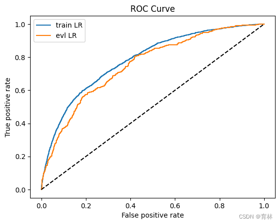
ROC曲线
描绘的是不同的截断点时,并以FPR和TPR为横纵坐标轴,描述随着截断点的变小,TPR随着FPR的变化。
纵轴:TPR=正例分对的概率 = TP/(TP+FN),其实就是查全率
横轴:FPR=负例分错的概率 = FP/(FP+TN)
作图步骤:
根据学习器的预测结果(注意,是正例的概率值,非0/1变量)对样本进行排序(从大到小)-----这就是截断点依次选取的顺序 按顺序选取截断点,并计算TPR和FPR—也可以只选取n个截断点,分别在1/n,2/n,3/n等位置 连接所有的点(TPR,FPR)即为ROC图
在这里插入代码片
KS值
作图步骤:
根据学习器的预测结果(注意,是正例的概率值,非0/1变量)对样本进行排序(从大到小)-----这就是截断点依次选取的顺序
按顺序选取截断点,并计算TPR和FPR —也可以只选取n个截断点,分别在1/n,2/n,3/n等位置
横轴为样本的占比百分比(最大100%),纵轴分别为TPR和FPR,可以得到KS曲线
TPR和FPR曲线分隔最开的位置就是最好的”截断点“,最大间隔距离就是KS值,通常>0.2即可认为模型有比较好偶的预测准确性。
y_pred = lr_model.predict_proba(x)[:,1]
fpr_lr_train,tpr_lr_train,_ = roc_curve(y,y_pred)
train_ks = abs(fpr_lr_train - tpr_lr_train).max()
print('train_ks : ',train_ks)y_pred = lr_model.predict_proba(val_x)[:,1]
fpr_lr,tpr_lr,_ = roc_curve(val_y,y_pred)
val_ks = abs(fpr_lr - tpr_lr).max()
print('val_ks : ',val_ks)from matplotlib import pyplot as plt
plt.plot(fpr_lr_train,tpr_lr_train,label = 'train LR')
plt.plot(fpr_lr,tpr_lr,label = 'evl LR')
plt.plot([0,1],[0,1],'k--')
plt.xlabel('False positive rate')
plt.ylabel('True positive rate')
plt.title('ROC Curve')
plt.legend(loc = 'best')
plt.show()
train_ks : 0.4151676259891534
val_ks : 0.3856283523530577
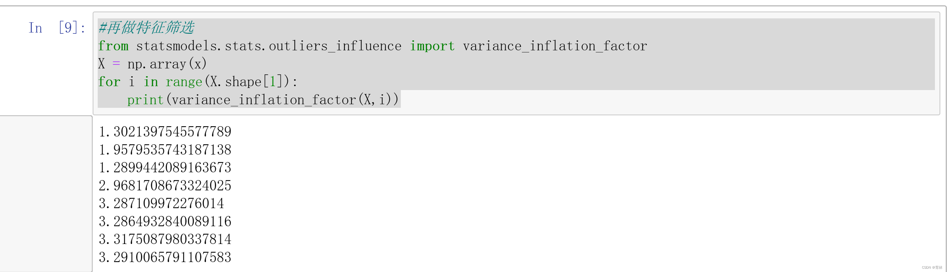
再做特征筛选
#再做特征筛选
from statsmodels.stats.outliers_influence import variance_inflation_factor
X = np.array(x)
for i in range(X.shape[1]):print(variance_inflation_factor(X,i))
import lightgbm as lgb
from sklearn.model_selection import train_test_split
train_x,test_x,train_y,test_y = train_test_split(x,y,random_state=0,test_size=0.2)
def  lgb_test(train_x,train_y,test_x,test_y):clf =lgb.LGBMClassifier(boosting_type = 'gbdt',objective = 'binary',metric = 'auc',learning_rate = 0.1,n_estimators = 24,max_depth = 5,num_leaves = 20,max_bin = 45,min_data_in_leaf = 6,bagging_fraction = 0.6,bagging_freq = 0,feature_fraction = 0.8,)clf.fit(train_x,train_y,eval_set = [(train_x,train_y),(test_x,test_y)],eval_metric = 'auc')return clf,clf.best_score_['valid_1']['auc'],
lgb_model , lgb_auc  = lgb_test(train_x,train_y,test_x,test_y)
feature_importance = pd.DataFrame({'name':lgb_model.booster_.feature_name(),'importance':lgb_model.feature_importances_}).sort_values(by=['importance'],ascending=False)
feature_importance

feature_lst = ['person_info','finance_info','credit_info','act_info']
x = train[feature_lst]
y = train['bad_ind']val_x =  val[feature_lst]
val_y = val['bad_ind']lr_model = LogisticRegression(C=0.1,class_weight='balanced')
lr_model.fit(x,y)
y_pred = lr_model.predict_proba(x)[:,1]
fpr_lr_train,tpr_lr_train,_ = roc_curve(y,y_pred)
train_ks = abs(fpr_lr_train - tpr_lr_train).max()
print('train_ks : ',train_ks)y_pred = lr_model.predict_proba(val_x)[:,1]
fpr_lr,tpr_lr,_ = roc_curve(val_y,y_pred)
val_ks = abs(fpr_lr - tpr_lr).max()
print('val_ks : ',val_ks)
from matplotlib import pyplot as plt
plt.plot(fpr_lr_train,tpr_lr_train,label = 'train LR')
plt.plot(fpr_lr,tpr_lr,label = 'evl LR')
plt.plot([0,1],[0,1],'k--')
plt.xlabel('False positive rate')
plt.ylabel('True positive rate')
plt.title('ROC Curve')
plt.legend(loc = 'best')
plt.show()
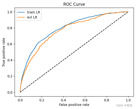
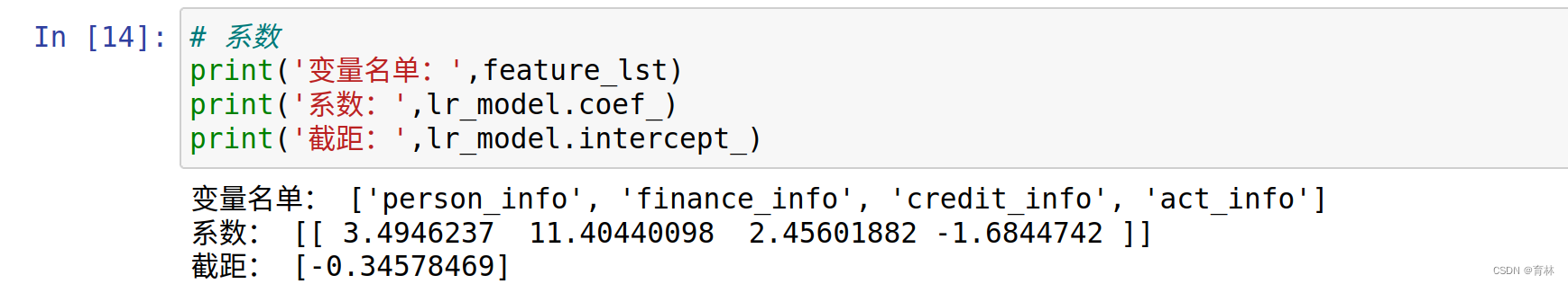
# 系数
print('变量名单:',feature_lst)
print('系数:',lr_model.coef_)
print('截距:',lr_model.intercept_)
生成报告
#生成报告
model = lr_model
row_num, col_num = 0, 0
bins = 20
Y_predict = [s[1] for s in model.predict_proba(val_x)]
Y = val_y
nrows = Y.shape[0]
lis = [(Y_predict[i], Y[i]) for i in range(nrows)]
ks_lis = sorted(lis, key=lambda x: x[0], reverse=True)
bin_num = int(nrows/bins+1)
bad = sum([1 for (p, y) in ks_lis if y > 0.5])
good = sum([1 for (p, y) in ks_lis if y <= 0.5])
bad_cnt, good_cnt = 0, 0
KS = []
BAD = []
GOOD = []
BAD_CNT = []
GOOD_CNT = []
BAD_PCTG = []
BADRATE = []
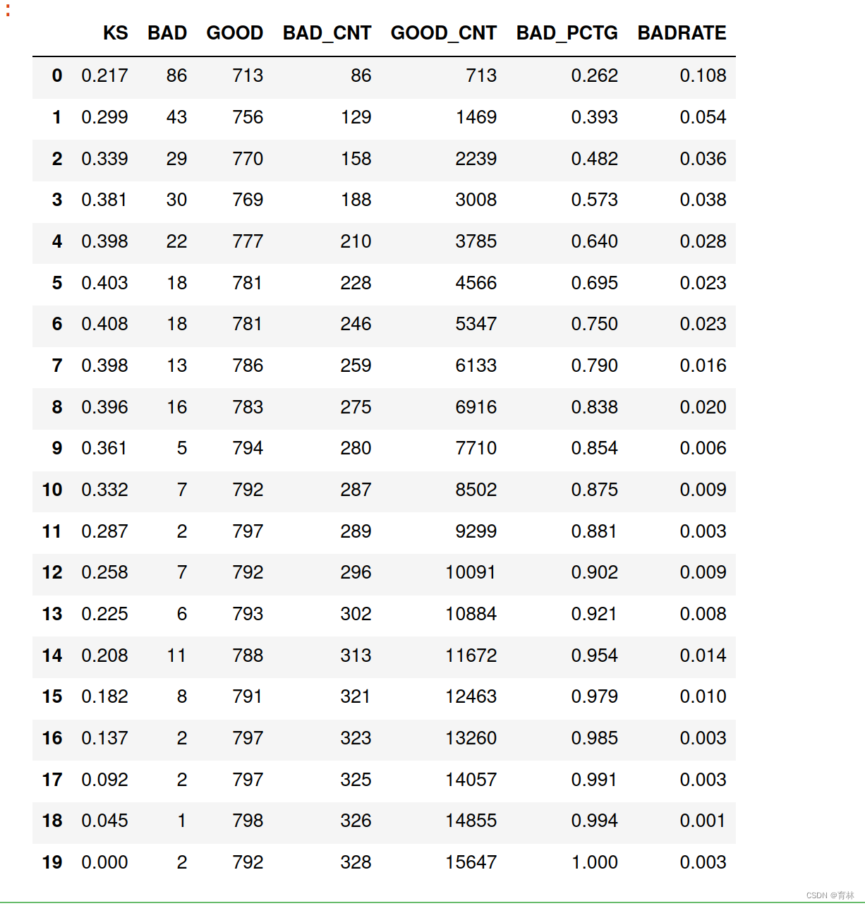
dct_report = {}
for j in range(bins):ds = ks_lis[j*bin_num: min((j+1)*bin_num, nrows)]bad1 = sum([1 for (p, y) in ds if y > 0.5])good1 = sum([1 for (p, y) in ds if y <= 0.5])bad_cnt += bad1good_cnt += good1bad_pctg = round(bad_cnt/sum(val_y),3)badrate = round(bad1/(bad1+good1),3)ks = round(math.fabs((bad_cnt / bad) - (good_cnt / good)),3)KS.append(ks)BAD.append(bad1)GOOD.append(good1)BAD_CNT.append(bad_cnt)GOOD_CNT.append(good_cnt)BAD_PCTG.append(bad_pctg)BADRATE.append(badrate)dct_report['KS'] = KSdct_report['BAD'] = BADdct_report['GOOD'] = GOODdct_report['BAD_CNT'] = BAD_CNTdct_report['GOOD_CNT'] = GOOD_CNTdct_report['BAD_PCTG'] = BAD_PCTGdct_report['BADRATE'] = BADRATE
val_repot = pd.DataFrame(dct_report)
val_repot
五、行为评分卡模型表现
from pyecharts.charts import *
from pyecharts import options as opts
from pylab import *
mpl.rcParams['font.sans-serif'] = ['SimHei']
np.set_printoptions(suppress=True)
pd.set_option('display.unicode.ambiguous_as_wide', True)
pd.set_option('display.unicode.east_asian_width', True)
line = (Line().add_xaxis(list(val_repot.index)).add_yaxis("分组坏人占比",list(val_repot.BADRATE),yaxis_index=0,color="red",).set_global_opts(title_opts=opts.TitleOpts(title="行为评分卡模型表现"),).extend_axis(yaxis=opts.AxisOpts(name="累计坏人占比",type_="value",min_=0,max_=0.5,position="right",axisline_opts=opts.AxisLineOpts(linestyle_opts=opts.LineStyleOpts(color="red")),axislabel_opts=opts.LabelOpts(formatter="{value}"),)).add_xaxis(list(val_repot.index)).add_yaxis("KS",list(val_repot['KS']),yaxis_index=1,color="blue",label_opts=opts.LabelOpts(is_show=False),)
)
line.render_notebook()

import seaborn as sns
sns.distplot(val.score,kde=True)val = val.sort_values('score',ascending=True).reset_index(drop=True)
df2=val.bad_ind.groupby(val['level']).sum()
df3=val.bad_ind.groupby(val['level']).count()
print(df2/df3)

总结
相关文章:
逻辑回归评分卡
文章目录 一、基础知识点(1)逻辑回归表达式(2)sigmoid函数的导数损失函数(Cross-entropy, 交叉熵损失函数)交叉熵求导准确率计算评估指标 二、导入库和数据集导入库读取数据 三、分析与训练四、模型评价ROC曲线KS值再做特征筛选生成报告 五、行为评分卡模型表现总结 一、基础知…...

DPDK系列之三十三DPDK并行机制的底层支持
一、背景介绍 在前面介绍了DPDK中的上层对并行的支持,特别是对多核的支持。但是,大家都知道,再怎么好的设计和架构,再优秀的编码,最终都要落到硬件和固件对整个上层应用的支持。单纯的硬件好处理,一个核不…...
LVGL_基础控件滚轮roller
LVGL_基础控件滚轮roller 1、创建滚轮roller控件 /* 创建一个 lv_roller 部件(对象) */ lv_obj_t * roller lv_roller_create(lv_scr_act()); // 创建一个 lv_roller 部件(对象),他的父对象是活动屏幕对象// 将部件(对象)添加到组,如果设置了默认组,…...
王道考研操作系统——文件管理
磁盘的基础知识 .txt用记事本这个应用程序打开,文件最重要的属性就是文件名了 保护信息:操作系统对系统当中的各个用户进行了分组,不同分组的用户对文件的操作权限是不一样的 文件的逻辑结构就是文件内部的数据/记录应该被怎么组织起来&…...

商业智能系统的主要功能包括数据仓库、数据ETL、数据统计输出、分析功能
ETL服务内容包含: 数据迁移数据合并数据同步数据交换数据联邦数据仓库...

基于帝国主义竞争优化的BP神经网络(分类应用) - 附代码
基于帝国主义竞争优化的BP神经网络(分类应用) - 附代码 文章目录 基于帝国主义竞争优化的BP神经网络(分类应用) - 附代码1.鸢尾花iris数据介绍2.数据集整理3.帝国主义竞争优化BP神经网络3.1 BP神经网络参数设置3.2 帝国主义竞争算…...

将python项目部署在一台服务器上
将python项目部署在一台服务器上 1.服务器2.部署方法2.1 手动部署2.2 容器化技术部署2.3 服务器less技术部署 1.服务器 服务器一般为:物理服务器和云服务器。 我的是物理服务器:这是将服务器硬件直接放置在您自己的数据中心或机房的传统方法。这种方法需…...
【C语言】善于利用指针(二)
💗个人主页💗 ⭐个人专栏——C语言初步学习⭐ 💫点击关注🤩一起学习C语言💯💫 目录 导读:1. 字符指针1.1 字符串的引用方式1.2 有趣的面试题 2. 数组指针2.1 一维数组指针的定义2.2 一维数组…...

Python调用C++
https://www.cnblogs.com/renfanzi/p/10276997.html Linux使用Python调用C/C接口(一) - 代码先锋网 linux系统上使用Python调用C生成的.so动态链接库opencv_linux 下python 编译为so ,给c使用_比赛学习者的博客-CSDN博客 https://www.cnblogs.com/shuimuqingyang/p/13618105…...

自己实现扫描全盘文件的函数。
1.自己实现扫描全盘的函数 def scan_disk(dir): global count,dir_count if os.path.isdir(dir): files os.listdir(dir) for file in files: print(file) dir_count 1 if os.path.isdir(dir os.sep file): …...

JSON文件读写
1、依赖文件 #include <QFile> #include <QJsonDocument> #include <QJsonObject> #include <QDebug> #include <QStringList>2、头文件 bool ReadJsonFile(const QString& filePath""); bool WriteJsonFile(const QString&…...
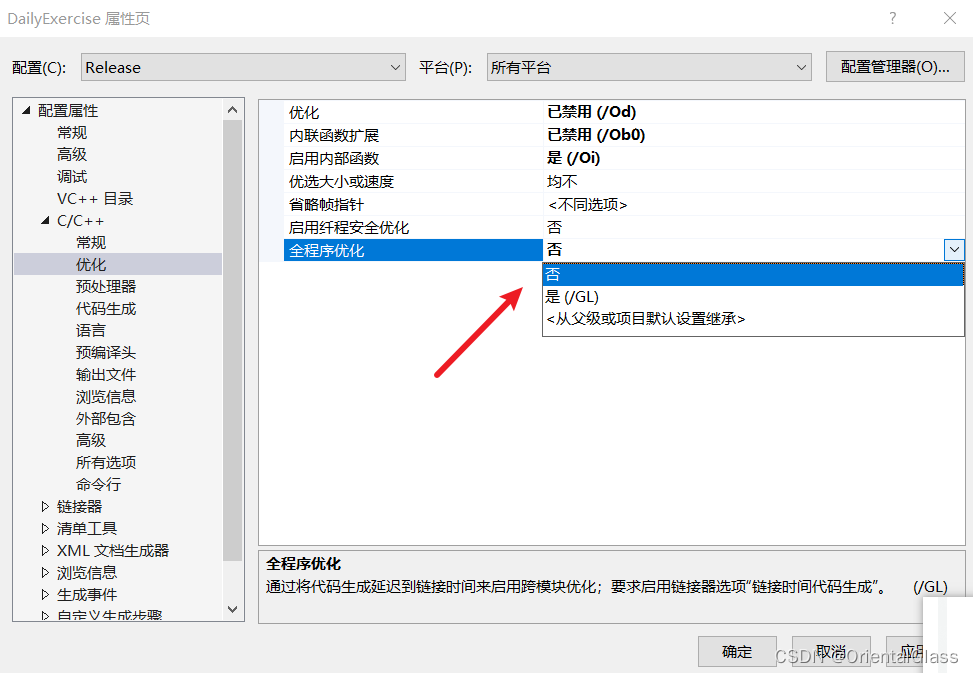
VisualStudio2022环境下Release模式编译dll无法使用TLS函数问题
Debug x86环境下正常使用TLS回调函数 切换到Release发现程序没有使用tls 到C/C > 优化中将全程序优化关闭即可...

ChatGPT基础使用总结
文章目录 一、ChatGPT基础概念大型语言模型LLMs---一种能够以类似人类语言的方式“说话”的软件ChatGPT定义---OpenAI 研发的一款聊天机器人程序(2022年GPT-3.5,属于大型语言模型)ChatGPT4.0---OpenAI推出了GPT系列的最新模型ChatGPT典型使用…...
解决报错: require is not defined in ES module scope
用node启动mjs文件报错:require is not defined in ES module scope 现象如下: 原因: 文件后缀是mjs, 被识别为es模块,但是node默认是commonjs格式,不支持也不能识别es模块。 解决办法:把文件后缀从.mjs改…...
STM32 10个工程篇:1.IAP远程升级(六)
在IAP远程升级的最后一篇博客里,笔者想概括性地梳理总结IAP程序设计中值得注意的问题,诚然市面上或者工作后存在不同版本的IAP下位机和上位机软件,也存在不同定义的报文格式,甚至对于相似的知识点不同教程又有着完全不同的解读&am…...

【智能家居项目】裸机版本——字体子系统 | 显示子系统
🐱作者:一只大喵咪1201 🐱专栏:《智能家居项目》 🔥格言:你只管努力,剩下的交给时间! 今天实现上图整个项目系统中的字体子系统和显示子系统。 目录 🀄设计思路…...

PDF中跳转到参考文献后,如何回到原文
在PDF中,点击了参考文献的超链接可以直接跳至参考文献的位置。 如果想从当前参考文献在回到正文中对应位置时,可以通过 Alt \red{\text{Alt}} Alt ← \red{\leftarrow} ← 实现。...

了解基于Elasticsearch 的站内搜索,及其替代方案
对于一家公司而言,数据量越来越多,如果快速去查找这些信息是一个很难的问题,在计算机领域有一个专门的领域IR(Information Retrival)研究如何获取信息,做信息检索。在国内的如百度这样的搜索引擎也属于这个…...

【多模态融合】TransFusion学习笔记(2)
接上篇【多模态融合】TransFusion学习笔记(1)。 从TransFusion-L到TransFusion ok,终于可以给出论文中那个完整的框架图了,我第一眼看到这个图有几个疑问: Q:Image Guidance这条虚线引出的Query Initialization是什么意思? Q:图像分支中的…...

Pyhon-每日一练(1)
🌈write in front🌈 🧸大家好,我是Aileen🧸.希望你看完之后,能对你有所帮助,不足请指正!共同学习交流. 🆔本文由Aileen_0v0🧸 原创 CSDN首发🐒 如…...

使用Nodejs和Taotoken为前端应用构建AI聊天后端
🚀 告别海外账号与网络限制!稳定直连全球优质大模型,限时半价接入中。 👉 点击领取海量免费额度 使用Node.js和Taotoken为前端应用构建AI聊天后端 基础教程类,指导前端或全栈开发者使用Node.js环境接入Taotoken&#…...

Windows 11优化终极指南:使用Win11Debloat一键提升电脑性能51%
Windows 11优化终极指南:使用Win11Debloat一键提升电脑性能51% 【免费下载链接】Win11Debloat A simple, lightweight PowerShell script that allows you to remove pre-installed apps, disable telemetry, as well as perform various other changes to declutte…...

如何轻松掌握开源OCR插件的实用技巧:5步快速上手指南
如何轻松掌握开源OCR插件的实用技巧:5步快速上手指南 【免费下载链接】Umi-OCR_plugins Umi-OCR 插件库 项目地址: https://gitcode.com/gh_mirrors/um/Umi-OCR_plugins 你是否曾被纸质文档的数字化问题困扰?或者需要从图片中提取数学公式却找不到…...

3步诊断Reloaded-II模组依赖无限下载循环:新手友好修复指南
3步诊断Reloaded-II模组依赖无限下载循环:新手友好修复指南 【免费下载链接】Reloaded-II Universal .NET Core Powered Modding Framework for any Native Game X86, X64. 项目地址: https://gitcode.com/gh_mirrors/re/Reloaded-II 如果你在使用Reloaded-I…...

别再为毕设供电发愁了!手把手教你用航模电池+降压模块搞定多电压系统
毕设供电系统实战指南:航模电池与智能降压方案全解析 刚拿到毕设题目的电子系学生小张,正盯着实验室桌上散落的传感器、单片机和电机发愁——这些设备需要的供电电压各不相同:单片机要7-12V,电机要12V,传感器却只要5V。…...

终极Windows安卓应用安装指南:告别模拟器,拥抱轻量级体验
终极Windows安卓应用安装指南:告别模拟器,拥抱轻量级体验 【免费下载链接】APK-Installer An Android Application Installer for Windows 项目地址: https://gitcode.com/GitHub_Trending/ap/APK-Installer 你是否厌倦了笨重的安卓模拟器&#x…...

如何快速掌握SRWE:Windows窗口分辨率自定义完整教程
如何快速掌握SRWE:Windows窗口分辨率自定义完整教程 【免费下载链接】SRWE Simple Runtime Window Editor 项目地址: https://gitcode.com/gh_mirrors/sr/SRWE 你是否曾遇到过游戏窗口大小不合适、截图分辨率不够高,或者想要为特定应用程序设置独…...

如何轻松解决软件授权难题?智能授权管理脚本全解析
如何轻松解决软件授权难题?智能授权管理脚本全解析 【免费下载链接】KMS_VL_ALL_AIO Smart Activation Script 项目地址: https://gitcode.com/gh_mirrors/km/KMS_VL_ALL_AIO 你是否曾经遇到过这样的情况:重要的办公软件突然提示授权过期…...

Nigate:让Mac与Windows硬盘和谐共处的开源桥梁
Nigate:让Mac与Windows硬盘和谐共处的开源桥梁 【免费下载链接】Free-NTFS-for-Mac Nigate: An open-source NTFS utility for Mac. It supports all Mac models (Intel and Apple Silicon), providing full read-write access, mounting, and management for NTFS …...

npcpy:模块化AI智能体框架,从角色构建到团队协作的工程实践
1. 项目概述:一个为AI应用构建者准备的“瑞士军刀”如果你和我一样,在过去几年里尝试过用大语言模型(LLM)构建点什么东西,那你大概率经历过这样的循环:从LangChain、LlamaIndex这类框架开始,被它…...