Applied Spatial Statistics(七):Python 中的空间回归
Applied Spatial Statistics(七):Python 中的空间回归
本笔记本演示了如何使用 pysal 的 spreg 库拟合空间滞后模型和空间误差模型。
- OLS
- 空间误差模型
- 空间滞后模型
- 三种模型的比较
- 探索滞后模型中的直接和间接影响
import numpy as np
import pandas as pdimport geopandas as gpd
import seaborn as sns
import matplotlib.pyplot as plt
from libpysal.weights import Queen
from splot.esda import plot_moran
from esda.moran import Moran
import spreg
1.数据
在此笔记本中,我将使用 2020 年美国总统选举数据集进行演示。
voting 数据框包含县级投票给民主党的人数百分比(编码为 new_pct_dem)以及该县的一些社会经济变量。该数据集仅包含美国本土 48 个州的统计数据。
voting = pd.read_csv('https://raw.github.com/Ziqi-Li/gis5122/master/data/voting_2020.csv')voting[['median_income']] = voting[['median_income']]/10000
voting.head()
| county_id | state | county | NAME | proj_X | proj_Y | total_pop | new_pct_dem | sex_ratio | pct_black | ... | median_income | pct_65_over | pct_age_18_29 | gini | pct_manuf | ln_pop_den | pct_3rd_party | turn_out | pct_fb | pct_uninsured | |
|---|---|---|---|---|---|---|---|---|---|---|---|---|---|---|---|---|---|---|---|---|---|
| 0 | 17051 | 17 | 51 | Fayette County, Illinois | 597979.5531 | 1796861.993 | 21565 | 18.445122 | 113.6 | 4.7 | ... | 4.6650 | 18.8 | 14.899142 | 0.4373 | 14.9 | 3.392715 | 1.923652 | 58.930984 | 1.3 | 8.2 |
| 1 | 17107 | 17 | 107 | Logan County, Illinois | 559814.6766 | 1920479.975 | 29003 | 29.420030 | 97.2 | 6.9 | ... | 5.7308 | 18.0 | 17.256836 | 0.4201 | 12.4 | 3.847224 | 2.332850 | 56.631552 | 1.6 | 4.5 |
| 2 | 17165 | 17 | 165 | Saline County, Illinois | 650278.3579 | 1660709.808 | 23994 | 25.601911 | 96.9 | 2.6 | ... | 4.4090 | 19.9 | 13.586730 | 0.4692 | 8.7 | 4.128654 | 1.778139 | 59.147937 | 1.0 | 4.2 |
| 3 | 17097 | 17 | 97 | Lake County, Illinois | 654010.9262 | 2174576.605 | 701473 | 62.275888 | 99.8 | 6.8 | ... | 8.9427 | 13.7 | 15.823132 | 0.4847 | 16.3 | 7.308201 | 1.954177 | 71.151975 | 18.7 | 6.8 |
| 4 | 17127 | 17 | 127 | Massac County, Illinois | 640398.9863 | 1599902.491 | 14219 | 25.626118 | 89.5 | 5.8 | ... | 4.7481 | 20.8 | 12.370772 | 0.4097 | 7.4 | 4.067788 | 1.396443 | 62.281425 | 1.0 | 5.4 |
5 rows × 22 columns
然后我们阅读了美国的县边界文件。
shp = gpd.read_file("https://raw.github.com/Ziqi-Li/gis5122/master/data/us_counties.geojson")
#Merge the shapefile with the voting data by the common county_id
shp_voting = shp.merge(voting, on ="county_id")#Dissolve the counties to obtain boundary of states, used for mapping
state = shp_voting.dissolve(by='STATEFP').geometry.boundary
选择本练习中要使用的变量,我从列表中选择了 6 个预测因子。
variable_names = ['sex_ratio', 'pct_black', 'pct_hisp','pct_bach', 'median_income','ln_pop_den']y = shp_voting[['new_pct_dem']].valuesX = shp_voting[variable_names].values
2.OLS model (baseline)
这里我演示如何使用 spring 来拟合 OLS 模型。当然你也可以使用 statsmodels。
#In the spreg.OLS() you need to specify the y and X, also variable names (optional)ols = spreg.OLS(y, X, name_y='new_pct_dem', name_x=variable_names)
print(ols.summary)
REGRESSION RESULTS
------------------SUMMARY OF OUTPUT: ORDINARY LEAST SQUARES
-----------------------------------------
Data set            :     unknown
Weights matrix      :        None
Dependent Variable  : new_pct_dem                Number of Observations:        3103
Mean dependent var  :     33.7616                Number of Variables   :           7
S.D. dependent var  :     16.2257                Degrees of Freedom    :        3096
R-squared           :      0.6091
Adjusted R-squared  :      0.6083
Sum squared residual:      319249                F-statistic           :    803.9833
Sigma-square        :     103.117                Prob(F-statistic)     :           0
S.E. of regression  :      10.155                Log likelihood        :  -11592.001
Sigma-square ML     :     102.884                Akaike info criterion :   23198.003
S.E of regression ML:     10.1432                Schwarz criterion     :   23240.284------------------------------------------------------------------------------------Variable     Coefficient       Std.Error     t-Statistic     Probability
------------------------------------------------------------------------------------CONSTANT         5.83676         1.96534         2.96984         0.00300sex_ratio         0.00613         0.01754         0.34970         0.72659pct_black         0.48310         0.01401        34.47681         0.00000pct_hisp         0.23952         0.01329        18.02612         0.00000pct_bach         0.97537         0.02854        34.17057         0.00000median_income        -1.66008         0.19755        -8.40329         0.00000ln_pop_den         2.13283         0.12925        16.50160         0.00000
------------------------------------------------------------------------------------REGRESSION DIAGNOSTICS
MULTICOLLINEARITY CONDITION NUMBER           33.073TEST ON NORMALITY OF ERRORS
TEST                             DF        VALUE           PROB
Jarque-Bera                       2        1166.636           0.0000DIAGNOSTICS FOR HETEROSKEDASTICITY
RANDOM COEFFICIENTS
TEST                             DF        VALUE           PROB
Breusch-Pagan test                6         268.617           0.0000
Koenker-Bassett test              6         118.745           0.0000
================================ END OF REPORT =====================================
我们可以与 statsmodels 进行比较,结果相同
查看 OLS 残差图
ols.u
array([[ 0.98102642],[-7.61122909],[ 3.44911401],...,[-3.82424613],[-0.7422498 ],[-1.11507546]])
from matplotlib import colors#For creating a discrete color classification
norm = colors.BoundaryNorm([-20, -10, -5, 0, 5, 10, 20],ncolors=256)ax = shp_voting.plot(column=ols.u.reshape(-1),legend=True,figsize=(15,8), norm=norm, linewidth=0.0)state.plot(ax=ax,linewidth=0.3,edgecolor="black")plt.title("Map of residuals of the OLS model",fontsize=15)
Text(0.5, 1.0, 'Map of residuals of the OLS model')
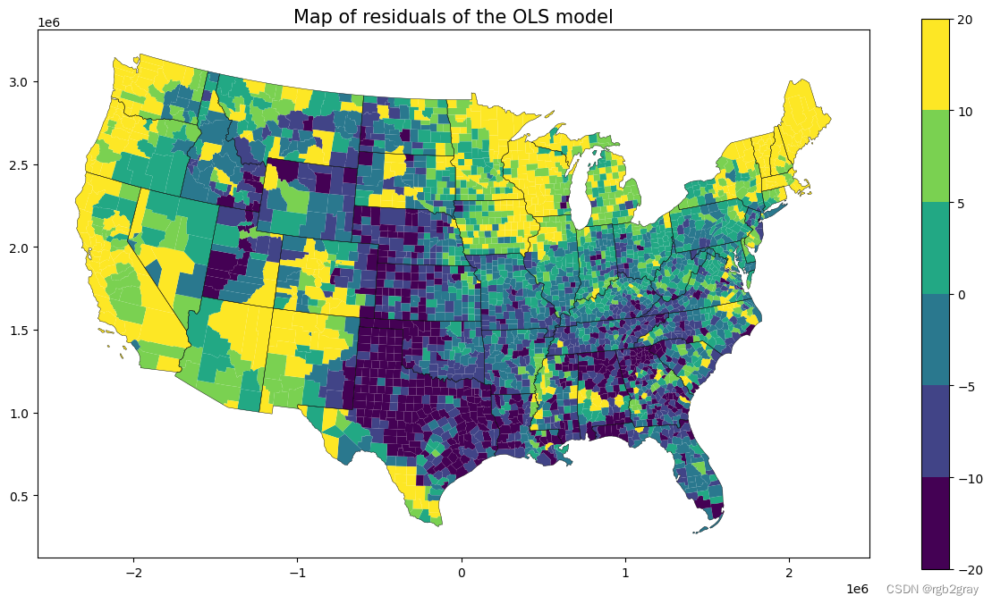
从 OLS 残差图中,我们可以看到空间自相关性很强,高/低残差聚集在一起。这强烈表明我们的模型缺少空间结构,并且违反了 OLS 的独立性假设。
然后让我们通过计算残差的 Moran’s I 来更定量地评估空间自相关性。
#Here we use the Queen contiguity
w = Queen.from_dataframe(shp_voting)#row standardization
w.transform = 'R'#The warning is saying there are two counties without neighbors, lets don't worry about this for now.
<ipython-input-14-9c7ca81e50b6>:2: FutureWarning: `use_index` defaults to False but will default to True in future. Set True/False directly to control this behavior and silence this warningw = Queen.from_dataframe(shp_voting)('WARNING: ', 2441, ' is an island (no neighbors)')
('WARNING: ', 2701, ' is an island (no neighbors)')/usr/local/lib/python3.10/dist-packages/libpysal/weights/weights.py:224: UserWarning: The weights matrix is not fully connected: There are 3 disconnected components.There are 2 islands with ids: 2441, 2701.warnings.warn(message)
#Here, lets calculate the Moran's I value, and plot it.
#ols.u is the residuals from the OLS modelols_moran = Moran(ols.u, w, permutations = 199) #199 permutationsplot_moran(ols_moran, figsize=(10,4))
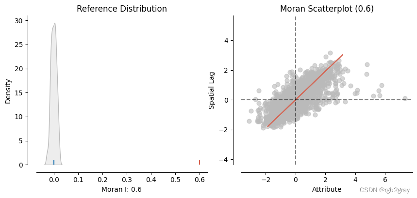
我们发现 Moran’s I 值等于 0.6,这让我们确信 OLS 残差图上确实存在很强的空间模式。
现在有两个选择:我们可以使用 滞后模型,或者我们可以使用 误差模型。
一个便利之处在于,如果您将权重矩阵传递给 OLS 函数,同时指定 spat_diag=True,那么您将获得一些额外的空间诊断,可以帮助您做出决定。如果您指定 moran=True,这还包括残差的 Moran’s I。
ols = spreg.OLS(y, X, w=w, spat_diag=True, moran=True,name_y='pct_dem', name_x=variable_names)print(ols.summary)
REGRESSION RESULTS
------------------SUMMARY OF OUTPUT: ORDINARY LEAST SQUARES
-----------------------------------------
Data set            :     unknown
Weights matrix      :     unknown
Dependent Variable  :     pct_dem                Number of Observations:        3103
Mean dependent var  :     33.7616                Number of Variables   :           7
S.D. dependent var  :     16.2257                Degrees of Freedom    :        3096
R-squared           :      0.6091
Adjusted R-squared  :      0.6083
Sum squared residual:      319249                F-statistic           :    803.9833
Sigma-square        :     103.117                Prob(F-statistic)     :           0
S.E. of regression  :      10.155                Log likelihood        :  -11592.001
Sigma-square ML     :     102.884                Akaike info criterion :   23198.003
S.E of regression ML:     10.1432                Schwarz criterion     :   23240.284------------------------------------------------------------------------------------Variable     Coefficient       Std.Error     t-Statistic     Probability
------------------------------------------------------------------------------------CONSTANT         5.83676         1.96534         2.96984         0.00300sex_ratio         0.00613         0.01754         0.34970         0.72659pct_black         0.48310         0.01401        34.47681         0.00000pct_hisp         0.23952         0.01329        18.02612         0.00000pct_bach         0.97537         0.02854        34.17057         0.00000median_income        -1.66008         0.19755        -8.40329         0.00000ln_pop_den         2.13283         0.12925        16.50160         0.00000
------------------------------------------------------------------------------------REGRESSION DIAGNOSTICS
MULTICOLLINEARITY CONDITION NUMBER           33.073TEST ON NORMALITY OF ERRORS
TEST                             DF        VALUE           PROB
Jarque-Bera                       2        1166.636           0.0000DIAGNOSTICS FOR HETEROSKEDASTICITY
RANDOM COEFFICIENTS
TEST                             DF        VALUE           PROB
Breusch-Pagan test                6         268.617           0.0000
Koenker-Bassett test              6         118.745           0.0000DIAGNOSTICS FOR SPATIAL DEPENDENCE
TEST                           MI/DF       VALUE           PROB
Moran's I (error)              0.6000        56.164           0.0000
Lagrange Multiplier (lag)         1        1952.063           0.0000
Robust LM (lag)                   1          18.792           0.0000
Lagrange Multiplier (error)       1        3119.345           0.0000
Robust LM (error)                 1        1186.074           0.0000
Lagrange Multiplier (SARMA)       2        3138.137           0.0000================================ END OF REPORT =====================================
从 L-M 检验中,我们可以预期误差模型比滞后模型更为合适(比较稳健得分:1186 比 18)。
3.Spatial Error Model (SEM)
现在让我们使用“spreg.ML_Error()”拟合空间错误模型,其中您需要指定 y、X 和权重矩阵 w。
sem = spreg.ML_Error(y, X, w=w, name_x=variable_names, name_y='new_pct_dem')print(sem.summary)
/usr/local/lib/python3.10/dist-packages/scipy/optimize/_minimize.py:913: RuntimeWarning: Method 'bounded' does not support relative tolerance in x; defaulting to absolute tolerance.warn("Method 'bounded' does not support relative tolerance in x; "REGRESSION RESULTS
------------------SUMMARY OF OUTPUT: ML SPATIAL ERROR (METHOD = full)
---------------------------------------------------
Data set            :     unknown
Weights matrix      :     unknown
Dependent Variable  : new_pct_dem                Number of Observations:        3103
Mean dependent var  :     33.7616                Number of Variables   :           7
S.D. dependent var  :     16.2257                Degrees of Freedom    :        3096
Pseudo R-squared    :      0.5167
Log likelihood      : -10170.5905
Sigma-square ML     :     33.4938                Akaike info criterion :   20355.181
S.E of regression   :      5.7874                Schwarz criterion     :   20397.462------------------------------------------------------------------------------------Variable     Coefficient       Std.Error     z-Statistic     Probability
------------------------------------------------------------------------------------CONSTANT        19.00473         1.49728        12.69280         0.00000sex_ratio        -0.04056         0.00988        -4.10353         0.00004pct_black         0.74856         0.01685        44.43261         0.00000pct_hisp         0.31866         0.01734        18.37383         0.00000pct_bach         0.72854         0.02000        36.42952         0.00000median_income        -2.42279         0.15714       -15.41832         0.00000ln_pop_den         1.83430         0.13375        13.71399         0.00000lambda         0.86984         0.00994        87.51130         0.00000
------------------------------------------------------------------------------------
================================ END OF REPORT =====================================
空间滞后误差项的 lambda(或其他使用 rho 的软件或符号)系数非常显著,并且其幅度相当大,这表明残差中存在很强的空间自相关性,这被滞后误差项捕获。
请注意,sem 的 sem.e_filtered 属性应该是 iid 误差。而 sem.u 是自回归误差 + iid 误差。现在让我们再次查看残差的 Moran’s I。
sem.e_filtered
array([[-2.82249844],[-2.93425648],[ 1.76293602],...,[ 0.58894001],[ 4.25853052],[-4.82251595]])
sem_moran = Moran(sem.e_filtered, w, permutations = 199) #199 permutations
plot_moran(sem_moran, zstandard=True, figsize=(10,4))
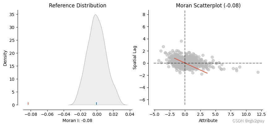
非常低的 Moran’s I -> 随机
ax = shp_voting.plot(column=sem.e_filtered.reshape(-1),legend=True,figsize=(15,8), norm=norm, linewidth=0.0)
state.plot(ax=ax,linewidth=0.3,edgecolor="black")
plt.title("Map of filtered residuals of the SEM model",fontsize=15)
Text(0.5, 1.0, 'Map of filtered residuals of the SEM model')
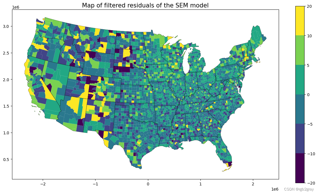
随机模式!太棒了!
4.Spatial Lag Model
类似地,让我们将此重复到空间滞后模型
slm = spreg.ML_Lag(y, X, w=w, name_y='new_pct_dem', name_x=variable_names)print(slm.summary)
REGRESSION RESULTS
------------------SUMMARY OF OUTPUT: MAXIMUM LIKELIHOOD SPATIAL LAG (METHOD = FULL)
-----------------------------------------------------------------
Data set            :     unknown
Weights matrix      :     unknown
Dependent Variable  : new_pct_dem                Number of Observations:        3103
Mean dependent var  :     33.7616                Number of Variables   :           8
S.D. dependent var  :     16.2257                Degrees of Freedom    :        3095
Pseudo R-squared    :      0.7744
Spatial Pseudo R-squared:  0.5591
Log likelihood      : -10853.5647
Sigma-square ML     :     59.4991                Akaike info criterion :   21723.129
S.E of regression   :      7.7136                Schwarz criterion     :   21771.450------------------------------------------------------------------------------------Variable     Coefficient       Std.Error     z-Statistic     Probability
------------------------------------------------------------------------------------CONSTANT         1.07097         1.50321         0.71245         0.47618sex_ratio         0.01044         0.01333         0.78274         0.43378pct_black         0.27765         0.01295        21.43381         0.00000pct_hisp         0.16619         0.01060        15.68552         0.00000pct_bach         0.83467         0.02200        37.93947         0.00000median_income        -2.99112         0.15043       -19.88429         0.00000ln_pop_den         1.47061         0.10082        14.58655         0.00000W_new_pct_dem         0.58112         0.01342        43.31362         0.00000
------------------------------------------------------------------------------------
================================ END OF REPORT =====================================
空间滞后项“W_new_pct_dem”的 rho 系数显著,且幅度很大,这表明因变量具有很强的空间溢出效应。
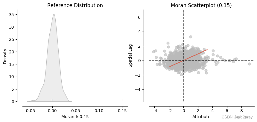
slm_moran = Moran(slm.u, w, permutations = 199) #199 permutations
plot_moran(slm_moran, zstandard=True, figsize=(10,4))
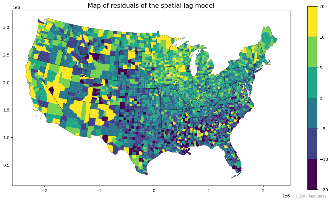
ax = shp_voting.plot(column=slm.u.reshape(-1),legend=True,figsize=(15,8), norm=norm, linewidth=0.0)state.plot(ax=ax,linewidth=0.3,edgecolor="black")
plt.title("Map of residuals of the spatial lag model",fontsize=15)
Text(0.5, 1.0, 'Map of residuals of the spatial lag model')
5.滞后、误差和 OLS 模型的交叉比较。
总体而言,我们看到尽管有一些变化(例如,在 SEM 模型中,%black 的影响更大),但估计值是一致的。OLS 模型不可靠,因为我们知道假设被违反了。在滞后模型中,即使我们考虑了邻近投票偏好,残差仍然显示出一些弱自相关性。而在误差模型中,我们确实观察到了随机残差。
所以如果我需要做出决定,我会使用误差模型。这也得到了 LM 测试的证据以及误差模型具有最低 AIC 值的支持。
| Predictor | OLS Estimates | SLM Estimates | SEM Estimates |
|---|---|---|---|
| CONSTANT | 5.83* | 1.07 | 19.00* |
| sex_ratio | 0.00 | 0.01 | -0.04* |
| pct_black | 0.48* | 0.27* | 0.74* |
| pct_hisp | 0.23* | 0.16* | 0.31* |
| pct_bach | 0.97* | 0.83* | 0.72* |
| median_income | -1.66* | -2.99* | -2.42* |
| ln_pop_den | 2.13* | 1.47* | 1.83* |
| lambda | NA | 0.58* | 0.86* |
| AIC | 23198.00 | 21723.12 | 20355.18 |
| Moran’s I of residuals | 0.60 | 0.15 | -0.08 |
6.更多关于 SLM 模型的内容:间接影响的检查。
场景:如果莱昂的 bach 百分比增加 1%,会怎样?附近县的 dem 百分比会发生什么变化?
步骤:
- 使用 w.full() 获取完整的 n x n 矩阵
- 计算 (I-pW)^-1*beta(此处的估计值是 SLM 模型中的 bach 百分比,因此为 0.83),现在您获得了完整的 n x n 变化交互。
- 找到任何感兴趣的县的行索引。
- 现在您可以选择该县的列并检查这将如何影响其他县。
#1.
w.full()[0]
array([[0., 0., 0., ..., 0., 0., 0.],[0., 0., 0., ..., 0., 0., 0.],[0., 0., 0., ..., 0., 0., 0.],...,[0., 0., 0., ..., 0., 0., 0.],[0., 0., 0., ..., 0., 0., 0.],[0., 0., 0., ..., 0., 0., 0.]])
np.identity(3103)
array([[1., 0., 0., ..., 0., 0., 0.],[0., 1., 0., ..., 0., 0., 0.],[0., 0., 1., ..., 0., 0., 0.],...,[0., 0., 0., ..., 1., 0., 0.],[0., 0., 0., ..., 0., 1., 0.],[0., 0., 0., ..., 0., 0., 1.]])
#2.
effects = np.linalg.inv(np.identity(3103) - 0.58*w.full()[0])*0.83 #n=3103, rho=0.58, est_pct_bach = 0.83effects
array([[8.92141250e-01, 1.32877317e-03, 1.52996497e-14, ...,3.14050249e-31, 5.12287114e-06, 1.79564935e-10],[9.49123691e-04, 8.98379566e-01, 1.43986921e-13, ...,4.16193409e-29, 1.14493906e-03, 1.32924287e-10],[1.27497081e-14, 1.67984741e-13, 9.03375896e-01, ...,8.63302503e-23, 5.33348558e-13, 2.63149009e-21],...,[2.61708541e-31, 4.85558978e-29, 8.63302503e-23, ...,8.88070682e-01, 8.55288372e-27, 1.32652812e-25],[3.65919367e-06, 1.14493906e-03, 4.57155907e-13, ...,7.33104319e-27, 8.95542764e-01, 4.10759600e-10],[1.12228084e-10, 1.16308751e-10, 1.97361756e-21, ...,9.94896087e-26, 3.59414650e-10, 9.05420698e-01]])
#3. find the row index for Leon, which is 67.
shp_voting[shp_voting['NAME_x'] == "Leon"]
| GEOID | STATEFP | NAME_x | county_id | geometry | state | county | NAME_y | proj_X | proj_Y | ... | median_income | pct_65_over | pct_age_18_29 | gini | pct_manuf | ln_pop_den | pct_3rd_party | turn_out | pct_fb | pct_uninsured | |
|---|---|---|---|---|---|---|---|---|---|---|---|---|---|---|---|---|---|---|---|---|---|
| 67 | 12073 | 12 | Leon | 12073 | POLYGON ((1080730.82089 870592.41110, 1086551.... | 12 | 73 | Leon County, Florida | 1.120705e+06 | 889449.6751 | ... | 5.3106 | 12.9 | 30.040722 | 0.4896 | 2.0 | 6.023568 | 1.202364 | 71.910474 | 6.8 | 8.1 |
| 1050 | 48289 | 48 | Leon | 48289 | POLYGON ((-30255.42040 920246.79226, -30598.62... | 48 | 289 | Leon County, Texas | 3.831304e+02 | 913423.2253 | ... | 4.3045 | 24.2 | 12.342525 | 0.5271 | 5.7 | 2.767577 | 0.899446 | 68.074417 | 5.2 | 17.0 |
2 rows × 26 columns
#Total effects for Leon can be obtained in the diagnoal of the full effects matrix.effects[67,67]
0.903899945968712
这表明,大学毕业生人数每增加 1%,民主党的投票份额将增加约 0.90%(直接 + 间接)。请注意,这大于滞后模型的系数(即 0.83),该系数仅捕捉直接影响。
间接影响是其自身与邻居之间的空间相互作用的结果,约为 0.07%(0.90 - 0.83)
现在让我们来看看莱昂的变化如何影响周边县市。
#get the effects for leon and plot it
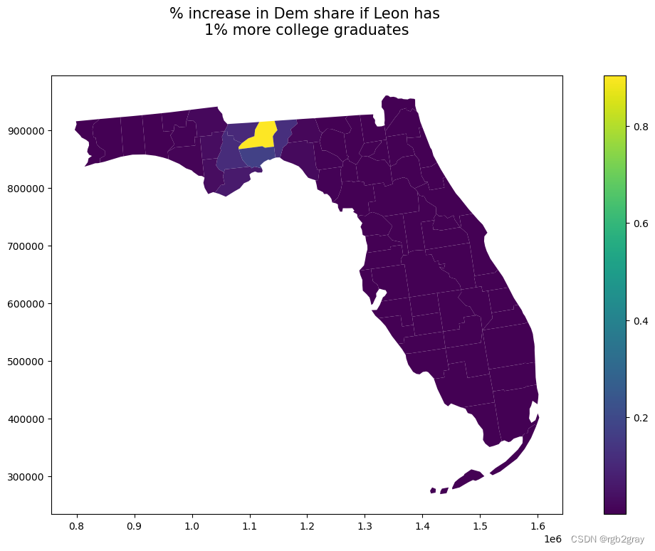
shp_voting['d_pct_bach_leon'] = effects[:,67]ax = shp_voting[shp_voting['state'] == 12].plot(column='d_pct_bach_leon',legend=True,figsize=(15,8), linewidth=0.0,aspect=1)plt.title("% increase in Dem share if Leon has \n1% more college graduates",fontsize=15,y=1.08)
Text(0.5, 1.08, '% increase in Dem share if Leon has \n1% more college graduates')
shp_voting[(shp_voting['state'] == 12) & (shp_voting['NAME_x'] == "Jefferson")].d_pct_bach_leon
2808    0.121902
Name: d_pct_bach_leon, dtype: float64
因此,我们基本上可以看出,如果莱昂的大学毕业生人数增加 1%,预计附近县的 %dem 份额将增加约 0.12%。例如,受莱昂变化的影响,杰斐逊县的 dem 份额可能会增加 0.12%。
shp_voting[(shp_voting['state'] == 12) & (shp_voting['NAME_x'] == "Miami-Dade")].d_pct_bach_leon
2607    1.163942e-08
Name: d_pct_bach_leon, dtype: float64
然而,我们可以看到,对于迈阿密戴德等较远的县,间接溢出效应基本为零。这是因为效应的幅度 (rho) 以及指定的 W 矩阵非常局部。
相关文章:
Applied Spatial Statistics(七):Python 中的空间回归
Applied Spatial Statistics(七):Python 中的空间回归 本笔记本演示了如何使用 pysal 的 spreg 库拟合空间滞后模型和空间误差模型。 OLS空间误差模型空间滞后模型三种模型的比较探索滞后模型中的直接和间接影响 import numpy as np impor…...
如何关闭软件开机自启,提升电脑开机速度?
如何关闭软件开机自启,提升电脑开机速度?大家知道,很多软件在安装时默认都会设置为开机自动启动。但是,有很多软件在我们开机之后并不是马上需要用到的,开机启动的软件过多会导致电脑开机变慢。那么,如何关…...

如何培养员工的竞争意识
一、背景 在当今快速变化的商业环境中,培养员工的竞争意识对于企业的长期成功至关重要。通过激发员工的竞争精神,企业能够提升整体绩效,增强创新能力,并在市场竞争中保持领先地位。本文将从多个方面探讨如何培养员工的竞争意识。 二、明确目标设定 设定清晰具体的目标:明…...

2025秋招NLP算法面试真题(二)-史上最全Transformer面试题:灵魂20问帮你彻底搞定Transformer
简单介绍 之前的20个问题的文章在这里: https://zhuanlan.zhihu.com/p/148656446 其实这20个问题不是让大家背答案,而是为了帮助大家梳理 transformer的相关知识点,所以你注意看会发现我的问题也是有某种顺序的。 本文涉及到的代码可以在…...
)
redis初步认识(一)
文章目录 概述安装编译 string数据结构基础命令应用对象存储累加器 list结构基础命令应用栈(先进后出FILO)队列 HASH基础命令存储结构应用存储对象 小结 概述 redis 是一个远程字典服务;当然,redis是内存数据库,kv数据库,最基础的…...

Android 开发必备知识点及面试题汇总(Android+Java+算法+性能优化+四大组件……
**虚引用:**顾名思义,就是形同虚设,如果一个对象仅持有虚引用,那么它相当于没有引用,在任何时候都可能被垃圾回收器回收。 7.介绍垃圾回收机制 **标记回收法:**遍历对象图并且记录可到达的对象,…...

安装Cmakeffmpeglibssh
首先安装cmake: sudo apt install cmake cmake --version然后这个输出正常就装好了 然后安装ffmpeg: tar xvzf n4.4.tar.gz cd FFmpeg-n4.4 chmod x configure ./configure --enable-gpl --enable-nonfree --enable-libx264 --enable-debug --disable-opti…...
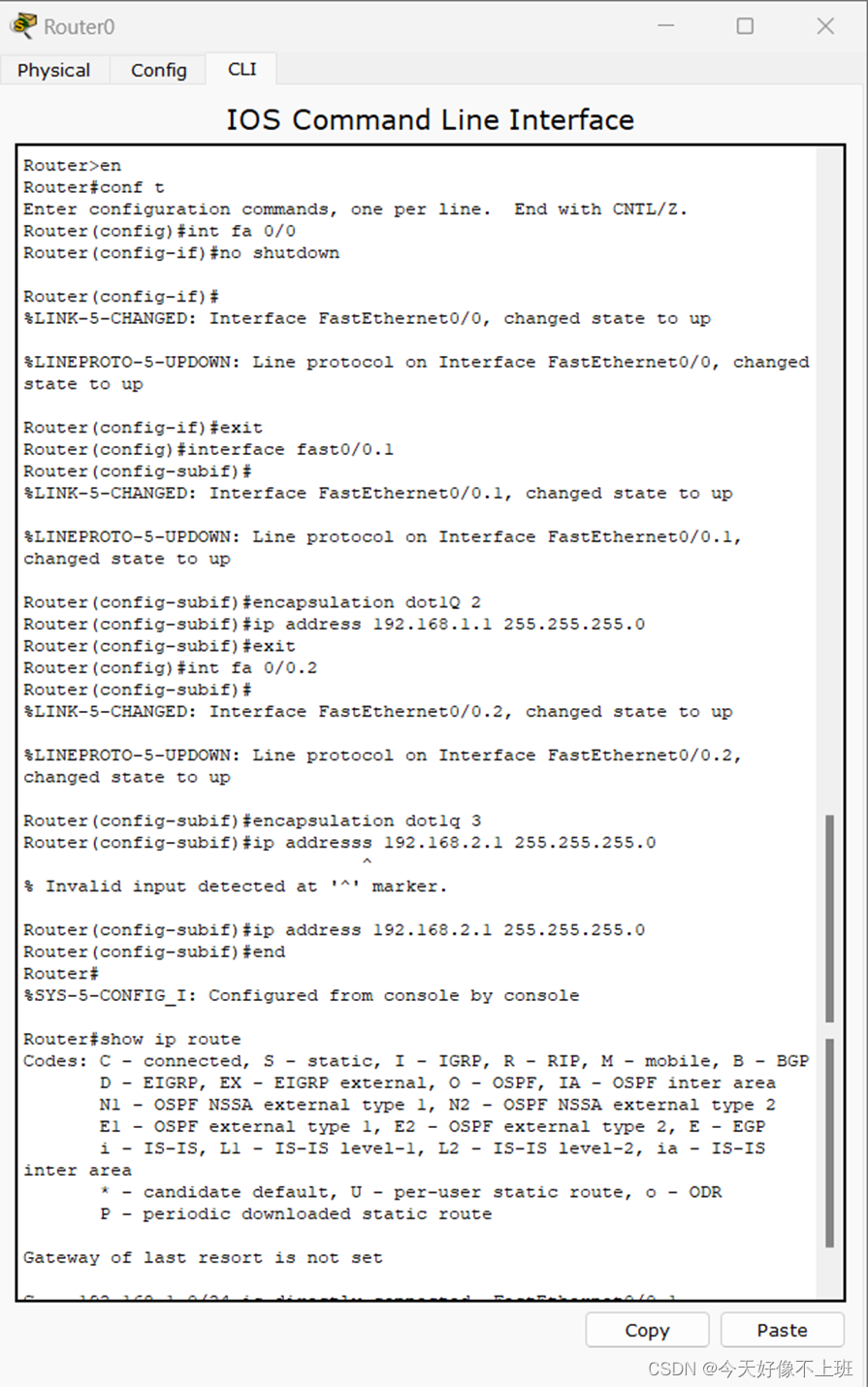
计算机网络实验(9):路由器的基本配置和单臂路由配置
一、 实验名称 路由器的基本配置和单臂路由配置 二、实验目的: (1)路由器的基本配置: 掌握路由器几种常用配置方法; 掌握采用Console线缆配置路由器的方法; 掌握采用Telnet方式配置路由器的方法&#…...

ArcGIS与Excel分区汇总统计三调各地类面积!数据透视表与汇总统计!
点击下方全系列课程学习 点击学习—>ArcGIS全系列实战视频教程——9个单一课程组合系列直播回放 点击学习——>遥感影像综合处理4大遥感软件ArcGISENVIErdaseCognition 01 需求说明 介绍一下ArcGIS与Excel统计分区各地类的三调地类面积。 ArcGIS统计分析不会&#x…...

QML 中宽度、高度与隐式宽度/高度的区别及其应用场景
在 QML 中,width、height 与 implicitWidth、implicitHeight 这几个属性常常令开发者感到困惑。本文将详细介绍它们之间的区别,并说明在何种情况下应使用隐式尺寸以及普通尺寸。 基本定义 width 和 height:表示组件/item 的实际尺寸。impli…...
解决事务管理中的方法调用问题)
如何利用AopContext.currentProxy()解决事务管理中的方法调用问题
在Spring应用开发中,使用AOP(面向切面编程)来管理事务是非常常见的做法。然而,在某些场景下,尤其是在同一个类的方法内部,一个非事务方法直接调用另一个带有事务注解的方法时,可能会遇到事务不生…...
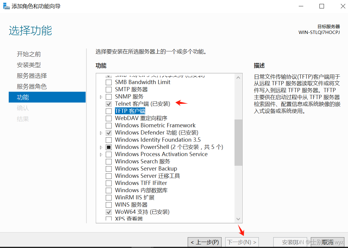
VMware虚拟机下载安装Windows Server 2016
「作者简介」:2022年北京冬奥会网络安全中国代表队,CSDN Top100,就职奇安信多年,以实战工作为基础对安全知识体系进行总结与归纳,著作适用于快速入门的 《网络安全自学教程》,内容涵盖系统安全、信息收集等…...
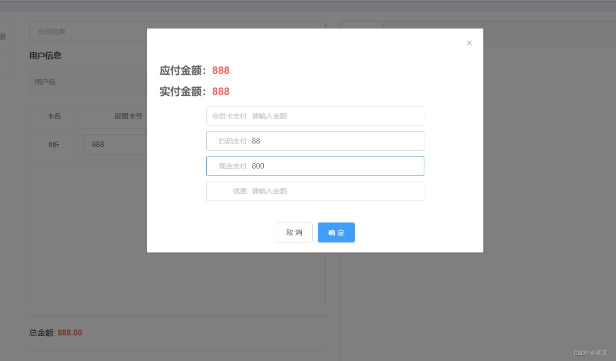
springboot vue 开源 会员收银系统 (7) 收银台的完善 新增开卡 结算
前言 完整版演示 开发版演示 在前面的开发中,我们成功完成了商品分类和商品信息的搭建,开发了收银台基础。现在,我们将进一步完善收银台的功能,添加开卡和结算功能,并在后台实现会员卡的创建和订单保存。同时ÿ…...
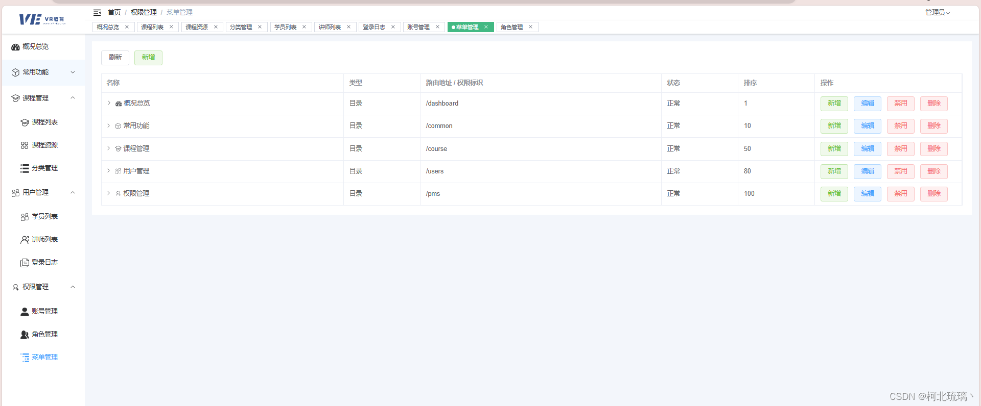
虚拟现实环境下的远程教育和智能评估系统(十三)
管理/教师端前端工作汇总education-admin: 首先是登录注册页面的展示 管理员 首页 管理员登录后的首页如下图所示 管理员拥有所有的权限 课程管理 1、可以查看、修改、增添、删除课程列表内容 2、可以对课程资源进行操作 3、可以对课程的类别信息进行管理&…...

深入了解软件设计模式:创新应用与优化代码结构
前言 在软件开发中,设计模式被广泛应用,通常分为三大类:创建型、结构型和行为型。这些模式经过时间验证,在解决特定问题和优化代码结构方面发挥了重要作用。本文将详细介绍每一类设计模式,并通过具体实例展示它们的应…...
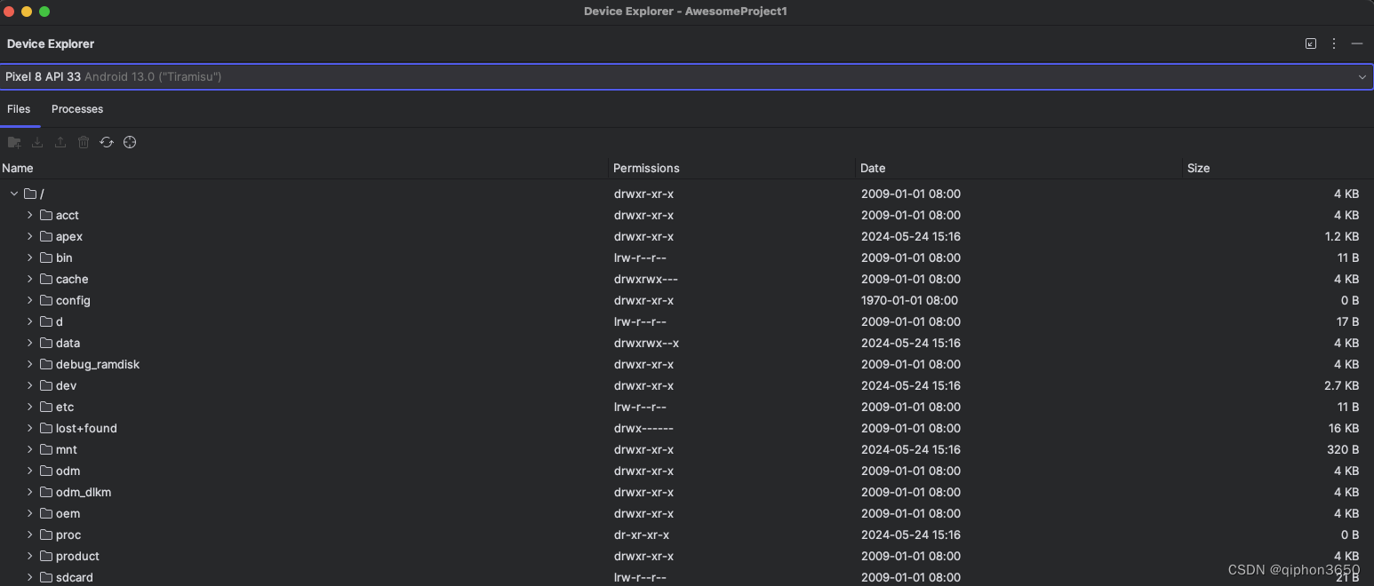
android studio 模拟器文件查找
android studio 模拟器文件查找 使用安卓模拟器下载文件后通常无法在系统硬盘上找到下载的文件,安卓 studio studio 其实提供了文件浏览工具,找到后可以直接使用 Android studio 打开 打开 Android studioview 菜单view > Tool Windows > Device…...
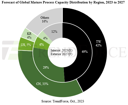
【科普】半导体制造过程的步骤、技术、流程
在这篇文章中,我们将学习基本的半导体制造过程。为了将晶圆转化为半导体芯片,它需要经历一系列复杂的制造过程,包括氧化、光刻、刻蚀、沉积、离子注入、金属布线、电气检测和封装等。 基本的半导体制造过程 1.晶圆(Wafer…...

c89、c99、c11
C99 标准开始引入了 // 单行注释。在此之前,C语言只支持 /* ... */ 多行注释。 具体说明: // 单行注释:在C99标准(ISO/IEC 9899:1999)引入之前,C语言中没有单行注释。C99标准借鉴了C的注释风格࿰…...
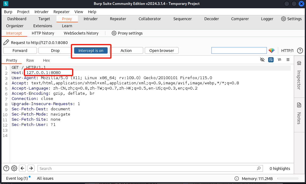
【网络安全的神秘世界】已解决burpsuite报错Failed to start proxy service on 127.0.0.1:8080
🌝博客主页:泥菩萨 💖专栏:Linux探索之旅 | 网络安全的神秘世界 | 专接本 | 每天学会一个渗透测试工具 解决burpsuite无法在 127.0.0.1:8080 上启动代理服务端口被占用以及抓不到本地包的问题 Burpsuite无法启动proxy…...

【C#】使用数字和时间方法ToString()格式化输出字符串显示
在C#编程项目开发中,几乎所有对象都有格式化字符串方法,其中常见的是数字和时间的格式化输出多少不一样,按实际需要而定吧,现记录如下,以后会用得上。 文章目录 数字格式化时间格式化 数字格式化 例如,保留…...

第08章 FastAPI 与 SSE 流式 RAG 后端
第08章 FastAPI 与 SSE 流式 RAG 后端 到目前为止,知识库、检索工具、MCP 客户端都已经就绪,但仍缺少一个面向最终用户的入口。本章用 FastAPI 把整条 RAG 链路串起来:接收前端发来的自然语言问题,调用 MCP 工具检索相关工单&…...

穿越机老鸟踩坑实录:MPU6000传感器在F4飞控上的IMU方向“玄学”配置
穿越机IMU方向配置实战:从MPU6000异常自旋到飞控底层校准 当你的穿越机在通电瞬间像被无形大手狠狠抽了一记耳光般疯狂自旋,而Betaflight地面站里陀螺仪数据却显示"一切正常"时,这往往意味着你正遭遇IMU方向配置的"量子纠缠态…...

STM32CubeMX外设配置实战——以F103C8T6的CAN与DMA为例
1. STM32CubeMX与F103C8T6开发基础 STM32CubeMX是ST官方推出的图形化配置工具,它能极大简化STM32系列MCU的外设初始化流程。对于刚接触STM32开发的工程师来说,这个工具就像"乐高积木说明书"——通过可视化操作就能完成80%的底层配置工作。我最…...

SAP KO88结算时,如何用BADI_FINS_ACDOC_POSTING_EVENTS把成本中心塞进自定义字段?
SAP KO88结算实战:通过BADI_FINS_ACDOC_POSTING_EVENTS实现成本中心到自定义字段的精准映射 在SAP工单结算(KO88)的复杂业务场景中,财务凭证的标准化字段往往无法满足企业多维度的分析需求。特别是当需要将特定成本中心信息映射到…...

SmarterRouter:基于软件定义与模块化构建智能路由器系统
1. 项目概述:一个更聪明的路由器,它到底想做什么?如果你和我一样,折腾过家里的网络,从刷第三方固件到组软路由,那你肯定对“路由器”这三个字有复杂的感情。它本该是默默无闻的网络基石,却常常因…...

如何快速免费管理游戏DLSS版本?DLSS Swapper终极指南
如何快速免费管理游戏DLSS版本?DLSS Swapper终极指南 【免费下载链接】dlss-swapper 项目地址: https://gitcode.com/GitHub_Trending/dl/dlss-swapper DLSS Swapper是一款革命性的开源工具,专为PC游戏玩家设计,能够智能管理、下载和…...

C++定时器避坑指南:线程安全、资源泄漏与时间轮参数怎么调?一次讲清楚
C定时器避坑指南:线程安全、资源泄漏与时间轮参数调优实战 在分布式系统和高并发场景中,定时器如同系统的心跳机制,其稳定性直接决定服务可靠性。去年某电商平台大促期间,由于定时任务堆积导致的雪崩效应,造成近千万损…...

基于Panel与LLM构建智能数据可视化应用的架构与实践
1. 项目概述与核心价值最近在数据可视化与交互应用开发领域,一个名为holoviz-topics/panel-chat-examples的项目仓库引起了我的注意。乍一看,这似乎只是将聊天界面(Chat Interface)与 Panel 这个强大的 Python 交互式仪表盘库结合…...
)
【仅剩217份】《Midjourney后印象派风格白皮书》V2.3——含17位艺术家专属LoRA适配建议、32组跨文化色彩映射表及实时风格强度校准工具(2024.06内部封测版)
更多请点击: https://intelliparadigm.com 第一章:后印象派风格的视觉基因与Midjourney语义解码 后印象派并非对自然的模仿,而是对色彩、结构与主观情绪的系统性重构——梵高旋转的星云、塞尚凝固的苹果、高更平面化的塔希提图腾,…...

KIVI开源工具箱:模块化设计赋能开发者效率提升
1. 项目概述:一个面向开发者的开源工具箱最近在GitHub上闲逛,发现了一个挺有意思的项目,叫KIVI。第一眼看到这个名字,我以为是某种新的UI框架或者设计系统,毕竟“KIVI”听起来有点像是“Kiwi”的变体,容易联…...