cs109-energy+哈佛大学能源探索项目 Part-2.1(Data Wrangling)
博主前期相关的博客见下:
cs109-energy+哈佛大学能源探索项目 Part-1(项目背景)
这次主要讲数据的整理。
Data Wrangling
数据整理
在哈佛的一些大型建筑中,有三种类型的能源消耗,电力,冷冻水和蒸汽。 冷冻水是用来冷却的,蒸汽是用来加热的。下图显示了哈佛工厂提供冷冻水和蒸汽的建筑。

Fig. Harvard chilled water and steam supply. (Left: chilled water, highlighted in blue. Right: Steam, highlighted in yellow)
图:哈佛的冷冻水和蒸汽供应。(左图:冷冻水,用蓝色突出显示。右边: 蒸汽,以黄色标示)。
我们选取了一栋建筑,得到了2011年07月01日至2014年10月31日的能耗数据。由于仪表故障,有几个月的数据丢失了。数据分辨率为每小时。在原始数据中,每小时的数据是仪表读数。为了得到每小时的消耗量,我们需要抵消数据,做减法。我们有从2012年1月到2014年10月每小时的天气和能源数据(2.75年)。这些天气数据来自剑桥的气象站。
在本节中,我们将完成以下任务。
1、从Harvard Energy Witness website上手动下载原始数据,获取每小时的电力、冷冻水和蒸汽。
2、清洁的天气数据,增加更多的功能,包括冷却度,加热度和湿度比。
3、根据假期、学年和周末估计每日入住率。
4、创建与小时相关的特征,即cos(hourOfDay 2 pi / 24)。
5、将电、冷冻水和蒸汽数据框与天气、时间和占用特性相结合。
数据下载
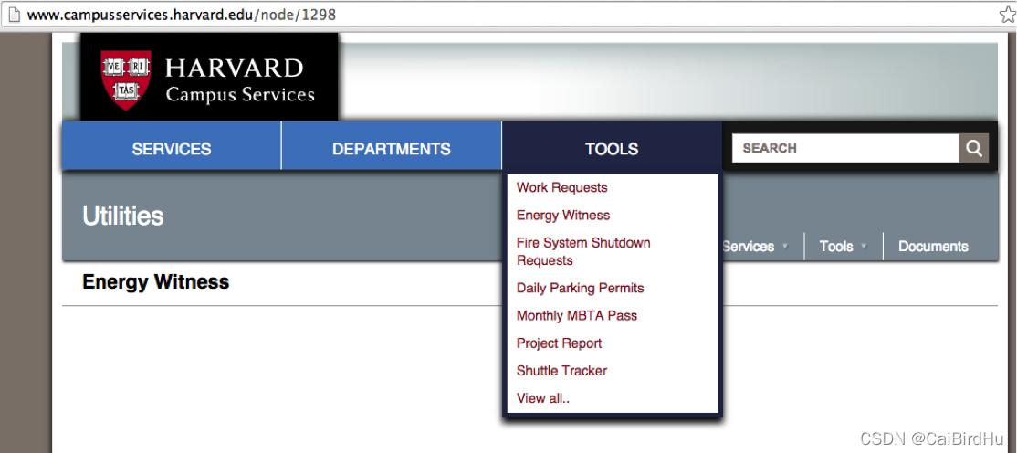
原始数据从(Harvard Energy Witness Website)下载
Energy Witness
PASS:该网站目前无法获取数据
后面部分主要学习其分析数据的技巧
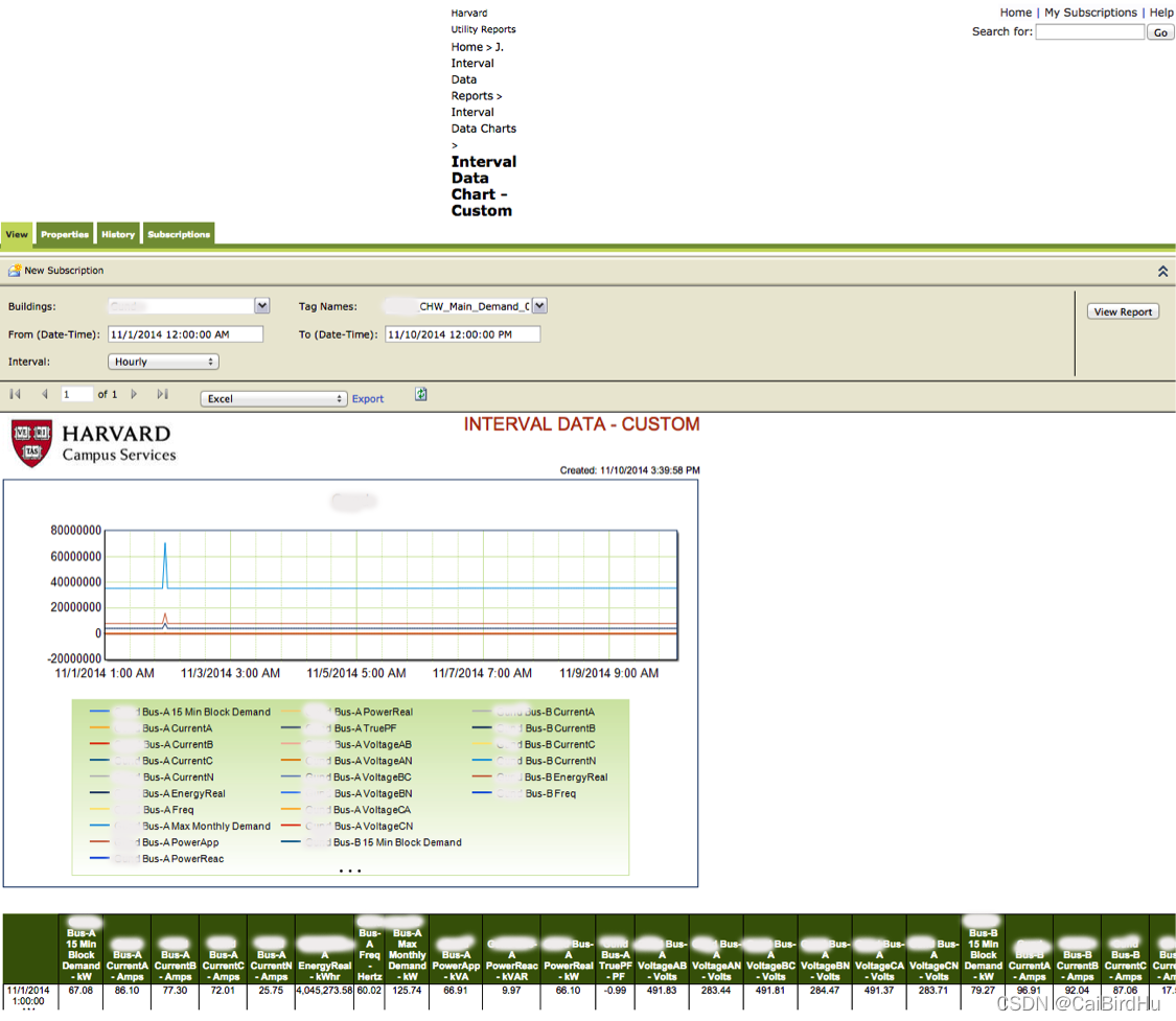
然后我们使用Pandas把它们放在 one dataframe。
file = 'Data/Org/0701-0930-2011.xls'
df = pd.read_excel(file, header = 0, skiprows = np.arange(0,6))files = ['Data/Org/1101-1130-2011.xls', 'Data/Org/1201-2011-0131-2012.xls','Data/Org/0201-0331-2012.xls','Data/Org/0401-0531-2012.xls','Data/Org/0601-0630-2012.xls','Data/Org/0701-0831-2012.xls','Data/Org/0901-1031-2012.xls','Data/Org/1101-1231-2012.xls','Data/Org/0101-0228-2013.xls','Data/Org/0301-0430-2013.xls','Data/Org/0501-0630-2013.xls','Data/Org/0701-0831-2013.xls','Data/Org/0901-1031-2013.xls','Data/Org/1101-1231-2013.xls','Data/Org/0101-0228-2014.xls','Data/Org/0301-0430-2014.xls', 'Data/Org/0501-0630-2014.xls', 'Data/Org/0701-0831-2014.xls','Data/Org/0901-1031-2014.xls']for file in files:data = pd.read_excel(file, header = 0, skiprows = np.arange(0,6))df = df.append(data)df.head()
这段代码的作用是将多个 Excel 文件中的数据读取到一个 DataFrame 中。首先,使用 Pandas 的 read_excel 函数读取 Data/Org/0701-0930-2011.xls 文件中的数据,并指定参数 header = 0 和 skiprows = np.arange(0,6),其中 header = 0 表示将第一行作为表头,skiprows = np.arange(0,6) 表示跳过前六行(通常是一些无用的信息或标题)。将读取的数据存储在 df 变量中。
接下来,定义了一个文件名列表 files,包含了要读取的所有 Excel 文件名。然后使用 for 循环逐一读取这些文件中的数据,将每个文件的数据存储在变量 data 中,再通过 append 方法将 data 中的数据添加到 df 变量中,最终得到一个包含所有文件数据的 DataFrame。
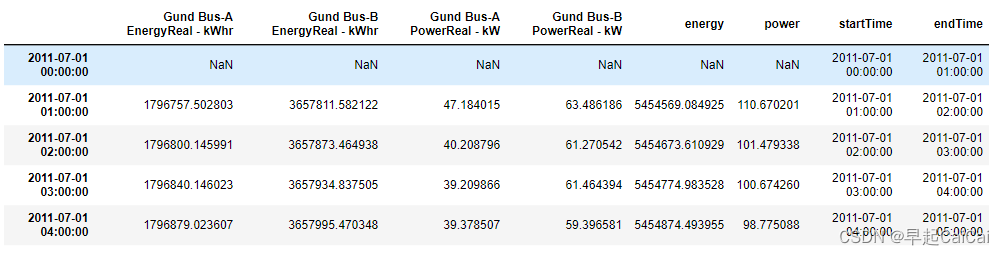
以上是原始的小时数据。
如你所见,非常混乱。移除无意义列的第一件事。
df.rename(columns={'Unnamed: 0':'Datetime'}, inplace=True)
nonBlankColumns = ['Unnamed' not in s for s in df.columns]
columns = df.columns[nonBlankColumns]
df = df[columns]
df = df.set_index(['Datetime'])
df.index.name = None
df.head()
这段代码做了以下事情:
- 将
Unnamed: 0'这一列的列名改为Datetime。 - 创建一个布尔列表 nonBlankColumns,其中包含所有列名中不包含
Unnamed的列。 - 选择所有布尔列表中为 True 的列名,并将其存储在一个新的 columns 变量中。
- 删除所有非空列(即 nonBlankColumns 中为 False 的列)。
- 将
Datetime列设置为索引。 - 将索引名称更改为 None。
- 返回 DataFrame 的前五行。
然后我们打印出所有的列名。只有少数几列是有用的,以获取每小时的电,冷冻水和蒸汽。
for item in df.columns:print item
Electricity
以电力为例,有两个计量器,“Gund Bus A"和"Gund Bus B”。"EnergyReal-kWhr"记录了累积用电量。我们不确定"PoweReal"确切代表什么。为了以防万一,我们也将其放入电力数据框中。
electricity=df[['Gund Bus-A EnergyReal - kWhr','Gund Bus-B EnergyReal - kWhr','Gund Bus-A PowerReal - kW','Gund Bus-B PowerReal - kW',]]
electricity.head()

Validate our data processing method by checking monthly energy consumption
通过月度能耗检查,验证数据处理方法
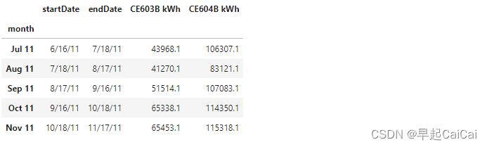
为了检验我们对数据的理解是否正确,我们想从小时数据计算出每月的用电量,然后将结果与facalities提供的每月数据进行比较,facalities也可以在Energy Witness上找到。
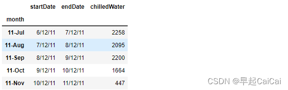
这是设施提供的月度数据,“Bus A和B”在这个月度表格中被称为“CE603B kWh”和“CE604B kWh”。它们只是两个电表。请注意,电表读数周期不是按照日历月计算的。
file = 'Data/monthly electricity.csv'
monthlyElectricityFromFacility = pd.read_csv(file, header=0)
monthlyElectricityFromFacility = monthlyElectricityFromFacility.set_index(['month'])
monthlyElectricityFromFacility.head()
这段代码用于读取一个名为 “monthly electricity.csv” 的文件,并将其转换为一个名为 monthlyElectricityFromFacility 的 Pandas 数据帧对象。在读取文件时,header=0参数表示将第一行视为数据帧的列标题。然后,将 “month” 列作为数据帧的索引列,使用 set_index() 方法来完成。最后,用 head() 方法来显示数据帧的前五行。
我们使用两个电表的“EnergyReal - kWhr”列。我们找到了电表读数周期的开始和结束日期的编号,然后用结束日期的编号减去开始日期的编号,就得到了每月的用电量。
monthlyElectricityFromFacility['startDate'] = pd.to_datetime(monthlyElectricityFromFacility['startDate'], format="%m/%d/%y")
values = monthlyElectricityFromFacility.index.valueskeys = np.array(monthlyElectricityFromFacility['startDate'])dates = {}
for key, value in zip(keys, values):dates[key] = valuesortedDates =  np.sort(dates.keys())
sortedDates = sortedDates[sortedDates > np.datetime64('2011-11-01')]months = []
monthlyElectricityOrg = np.zeros((len(sortedDates) - 1, 2))
for i in range(len(sortedDates) - 1):begin = sortedDates[i]end = sortedDates[i+1]months.append(dates[sortedDates[i]])monthlyElectricityOrg[i, 0] = (np.round(electricity.loc[end,'Gund Bus-A EnergyReal - kWhr'] -  electricity.loc[begin,'Gund Bus-A EnergyReal - kWhr'], 1))monthlyElectricityOrg[i, 1] = (np.round(electricity.loc[end,'Gund Bus-B EnergyReal - kWhr'] -  electricity.loc[begin,'Gund Bus-B EnergyReal - kWhr'], 1))monthlyElectricity = pd.DataFrame(data = monthlyElectricityOrg, index = months, columns = ['CE603B kWh', 'CE604B kWh'])plt.figure()
fig, ax = plt.subplots()
fig = monthlyElectricity.plot(marker = 'o', figsize=(15,6), rot = 40, fontsize = 13, ax = ax, linestyle='')
fig.set_axis_bgcolor('w')
plt.xlabel('Billing month', fontsize = 15)
plt.ylabel('kWh', fontsize = 15)
plt.tick_params(which=u'major', reset=False, axis = 'y', labelsize = 13)
plt.xticks(np.arange(0,len(months)),months)
plt.title('Original monthly consumption from hourly data',fontsize = 17)text = 'Meter malfunction'
ax.annotate(text, xy = (9, 4500000), xytext = (5, 2), fontsize = 15,textcoords = 'offset points', ha = 'center', va = 'top')ax.annotate(text, xy = (8, -4500000), xytext = (5, 2), fontsize = 15, textcoords = 'offset points', ha = 'center', va = 'bottom')ax.annotate(text, xy = (14, -2500000), xytext = (5, 2), fontsize = 15, textcoords = 'offset points', ha = 'center', va = 'bottom')ax.annotate(text, xy = (15, 2500000), xytext = (5, 2), fontsize = 15, textcoords = 'offset points', ha = 'center', va = 'top')plt.show()
以下是代码的解释:
monthlyElectricityFromFacility['startDate'] = pd.to_datetime(monthlyElectricityFromFacility['startDate'], format="%m/%d/%y")
将monthlyElectricityFromFacility数据框中的"startDate"列转换为datetime类型,并指定日期格式为"%m/%d/%y"。
values = monthlyElectricityFromFacility.index.values
keys = np.array(monthlyElectricityFromFacility['startDate'])
将monthlyElectricityFromFacility数据框的索引值保存到values中,并将"startDate"列的值保存到keys中。
dates = {}
for key, value in zip(keys, values):dates[key] = value
创建一个名为dates的字典,将"startDate"列的值作为键,索引值作为值存储到dates字典中。
sortedDates =  np.sort(dates.keys())
sortedDates = sortedDates[sortedDates > np.datetime64('2011-11-01')]
将dates字典的键按升序排序,并将排序后的结果保存到sortedDates中,然后从排序后的结果中筛选出大于2011年11月1日的日期。
months = []
monthlyElectricityOrg = np.zeros((len(sortedDates) - 1, 2))
for i in range(len(sortedDates) - 1):begin = sortedDates[i]end = sortedDates[i+1]months.append(dates[sortedDates[i]])monthlyElectricityOrg[i, 0] = (np.round(electricity.loc[end,'Gund Bus-A EnergyReal - kWhr'] -  electricity.loc[begin,'Gund Bus-A EnergyReal - kWhr'], 1))monthlyElectricityOrg[i, 1] = (np.round(electricity.loc[end,'Gund Bus-B EnergyReal - kWhr'] -  electricity.loc[begin,'Gund Bus-B EnergyReal - kWhr'], 1))
创建一个空列表months和一个形状为(len(sortedDates) - 1, 2)的全零数组monthlyElectricityOrg。然后遍历sortedDates中的每个日期,计算开始日期和结束日期之间的用电量,并将用电量保存到monthlyElectricityOrg数组中。同时,将每个月的名称保存到months列表中。
monthlyElectricity = pd.DataFrame(data = monthlyElectricityOrg, index = months, columns = ['CE603B kWh', 'CE604B kWh'])
将monthlyElectricityOrg数组转换为数据框,并将months列表作为索引,[‘CE603B kWh’, ‘CE604B kWh’]作为列名。
plt.figure()
fig, ax = plt.subplots()
fig = monthlyElectricity.plot(marker = 'o', figsize=(15,6), rot = 40, fontsize = 13, ax = ax, linestyle='')
fig.set_axis_bgcolor('w')
plt.xlabel('Billing month', fontsize = 15)
plt.ylabel('kWh', fontsize = 15)
plt.tick_params(which=u'major', reset=False, axis = 'y', labelsize = 13)
plt.xticks(np.arange(0,len(months)),months)
plt.title('Original monthly consumption from hourly data',fontsize = 17)
创建一个图形,并绘制monthlyElectricity数据框中的数据。设置x轴标签为"Billing month",y轴标签为"kWh",设置y轴标签字体大小为15。设置y轴刻度标签的字体大小为13,设置x轴刻度标签为months列表中的月份名称,并将x轴刻度标签旋转40度。设置图形标题为"Original monthly consumption from hourly data",字体大小为17。
text = 'Meter malfunction'
ax.annotate(text, xy = (9, 4500000), xytext = (5, 2), fontsize = 15,textcoords = 'offset points', ha = 'center', va = 'top')ax.annotate(text, xy = (8, -4500000), xytext = (5, 2), fontsize = 15, textcoords = 'offset points', ha = 'center', va = 'bottom')ax.annotate(text, xy = (14, -2500000), xytext = (5, 2), fontsize = 15, textcoords = 'offset points', ha = 'center', va = 'bottom')ax.annotate(text, xy = (15, 2500000), xytext = (5, 2), fontsize = 15, textcoords = 'offset points', ha = 'center', va = 'top')
在图形上添加四个文本注释,分别位于坐标点(9, 4500000)、(8, -4500000)、(14, -2500000)和(15, 2500000)处,文本内容为"Meter malfunction",字体大小为15,注释框的位置偏移量为(5, 2)。
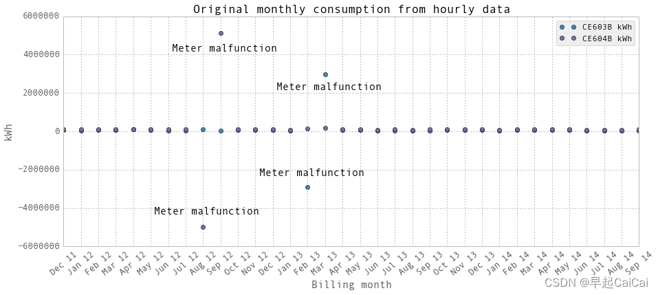
上面是使用我们的数据处理方法绘制的月度用电量图。显然,两个电表在几个月内发生了故障。图中有两组点,分别来自于两个电表,分别标注为"CE603B"和"CE604B"。建筑物的总用电量是这两个电表的电量之和。
图中的4个离群点为异常点
monthlyElectricity.loc['Aug 12','CE604B kWh'] = np.nan
monthlyElectricity.loc['Sep 12','CE604B kWh'] = np.nan
monthlyElectricity.loc['Feb 13','CE603B kWh'] = np.nan
monthlyElectricity.loc['Mar 13','CE603B kWh'] = np.nanfig,ax = plt.subplots(1, 1,figsize=(15,8))
#ax.set_axis_bgcolor('w')
plt.bar(np.arange(0, len(monthlyElectricity))-0.5,monthlyElectricity['CE603B kWh'], label='Our data processing from hourly data')
plt.plot(monthlyElectricityFromFacility.loc[months,'CE603B kWh'],'or', label='Facility data')
plt.xticks(np.arange(0,len(months)),months)
plt.xlabel('Month',fontsize=15)
plt.ylabel('kWh',fontsize=15)
plt.xlim([0, len(monthlyElectricity)])
plt.legend()
ax.set_xticklabels(months, rotation=40, fontsize=13)
plt.tick_params(which=u'major', reset=False, axis = 'y', labelsize = 15)
plt.title('Comparison between our data processing and facilities, Meter CE603B',fontsize=20)text = 'Meter malfunction \n estimated by facility'
ax.annotate(text, xy = (14, monthlyElectricityFromFacility.loc['Feb 13','CE603B kWh']), xytext = (5, 50), fontsize = 15, arrowprops=dict(facecolor='black', shrink=0.15),textcoords = 'offset points', ha = 'center', va = 'bottom')ax.annotate(text, xy = (15, monthlyElectricityFromFacility.loc['Mar 13','CE603B kWh']), xytext = (5, 50), fontsize = 15, arrowprops=dict(facecolor='black', shrink=0.15),textcoords = 'offset points', ha = 'center', va = 'bottom')
plt.show()fig,ax = plt.subplots(1, 1,figsize=(15,8))
#ax.set_axis_bgcolor('w')
plt.bar(np.arange(0, len(monthlyElectricity))-0.5, monthlyElectricity['CE604B kWh'], label='Our data processing from hourly data')
plt.plot(monthlyElectricityFromFacility.loc[months,'CE604B kWh'],'or', label='Facility data')
plt.xticks(np.arange(0,len(months)),months)
plt.xlabel('Month',fontsize=15)
plt.ylabel('kWh',fontsize=15)
plt.xlim([0, len(monthlyElectricity)])
plt.legend()
ax.set_xticklabels(months, rotation=40, fontsize=13)
plt.tick_params(which=u'major', reset=False, axis = 'y', labelsize = 15)
plt.title('Comparison between our data processing and facilities, Meter CE604B',fontsize=20)ax.annotate(text, xy = (9, monthlyElectricityFromFacility.loc['Sep 12','CE604B kWh']), xytext = (5, 50), fontsize = 15, arrowprops=dict(facecolor='black', shrink=0.15),textcoords = 'offset points', ha = 'center', va = 'bottom')ax.annotate(text, xy = (8, monthlyElectricityFromFacility.loc['Aug 12','CE604B kWh']), xytext = (5, 50), fontsize = 15, arrowprops=dict(facecolor='black', shrink=0.15),textcoords = 'offset points', ha = 'center', va = 'bottom')
plt.show()
这段代码的功能是绘制两个柱状图,比较我们的数据处理结果和设施提供的数据之间的差异。具体来说:
- 四行代码用于将一些数据设置为缺失值,以标识某些时间点上的电表故障。
- 第一个柱状图绘制了CE603B电表的用电量数据,并在每个月份的柱状图上标出了相应的数据点。同时,使用红色圆圈标识了设施提供的CE603B电表的用电量数据。x轴标签为月份,y轴标签为kWh。
- 第二个柱状图绘制了CE604B电表的用电量数据,并在每个月份的柱状图上标出了相应的数据点。同时,使用红色圆圈标识了设施提供的CE604B电表的用电量数据。x轴标签为月份,y轴标签为kWh。
每个图形中,文本注释用于标识某些数据点对应的电表故障,箭头指向相应的故障数据点。
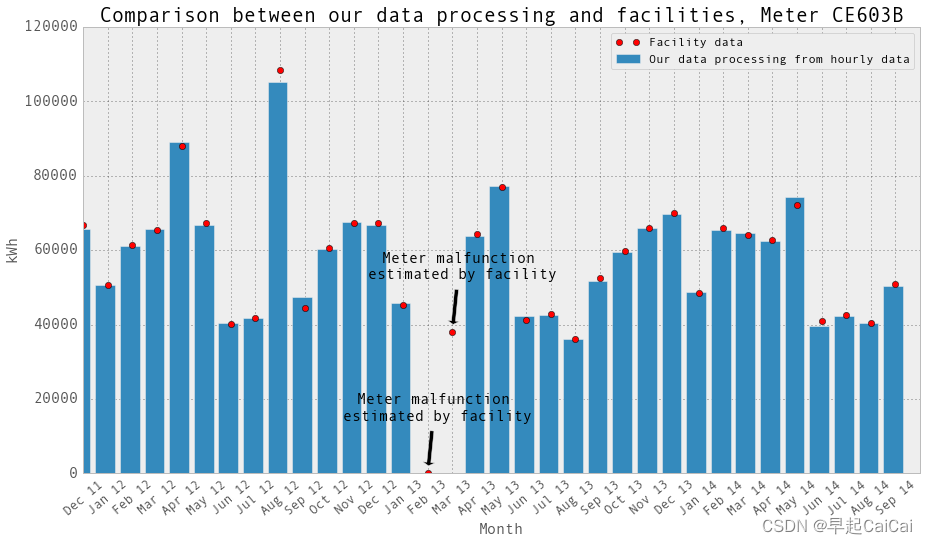
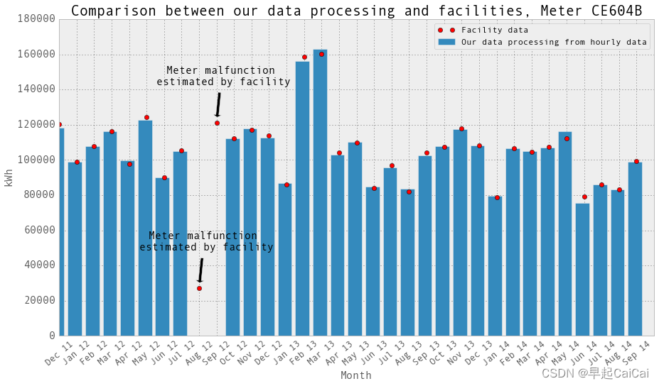
这张图片中的点是设施提供的月度数据。它们是账单上的数字。当电表发生故障时,设施会估算用电量以进行计费。我们在绘图中排除的数据点不在图中。它们的用电量远高于正常水平(比其他正常用电量高出30倍)。 “Meter malfunction, estimated by facility” 意味着在这个月,电表出现故障,这个点是设施估算的结果。
CE603B电表在2013年2月和3月发生了故障。CE604B电表在2012年8月和9月发生了故障。我们将这些月份的数据设置为np.nan,并将它们从回归中排除。再次绘制柱状图并与设施提供的月度数据进行比较。它们吻合!当然,除了电表发生故障的那些月份。在这些月份,设施估算用电量以进行计费。对于我们来说,在回归中我们只是排除了这些月份的小时和日数据点。
建筑物的总用电量是这两个电表的电量之和。为了确保准确性,我们保留了“功率”数据并将其与“能量”数据进行比较。
electricity['energy'] = electricity['Gund Bus-A EnergyReal - kWhr'] + electricity['Gund Bus-B EnergyReal - kWhr']
electricity['power'] = electricity['Gund Bus-A PowerReal - kW'] + electricity['Gund Bus-B PowerReal - kW']
electricity.head()
Derive hourly consumption
计算每小时用电量
计算每小时用电量的方法是,下一个小时的电表度数减去当前小时的电表度数,即"energy"列中下一个小时的数值减去当前小时的数值。我们假设电表度数是在小时结束时记录的。为了避免混淆,我们在数据框中还标记了电表读数的开始时间和结束时间。我们比较了下一个小时的功率数据和计算得到的每小时用电量,大部分情况下,功率和每小时用电量相差不大。但有时候有很大的差异。
电表记录的是累积用电量。例如,今天开始时,电表度数为10。一个小时后,用电量为1,那么电表读数就加一变为11,以此类推。因此,电表读数应该一直在增加。然而,我们发现有时电表读数会突然掉到0,然后过了一段时间后再次变成很高的正数。这会导致负的每小时用电量,然后是荒谬的极高的正数。我们通过计算t + 1时刻的电表读数 - t时刻的电表读数来获取每小时/每日的用电量。如果结果是负数或荒谬地高,我们就认为电表发生了故障。现在我们将这些数据点设置为np.nan。通过查看电子表格中的原始数据和月度绘图,我们确定了电表故障的确切日期。
此外,有时会出现比正常值高出千倍的荒谬数据点。正常的每小时用电量范围在100至400之间。我们创建了一个过滤器:index = abs(hourlyEnergy) < 200000,这意味着只有低于200000的值才会被保留。
# In case there are any missing hours, reindex to get the entire time span. Fill in nan data.
hourlyTimestamp = pd.date_range(start = '2011/7/1', end = '2014/10/31', freq = 'H')# Somehow, reindex does not work well. October 2011 and several other hours are missing.
# Basically it is just the length of original length.
#electricity.reindex(hourlyTimestamp, inplace = True, fill_value = np.nan)startTime = hourlyTimestamp
endTime = hourlyTimestamp + np.timedelta64(1,'h')
hourlyTime = pd.DataFrame(data = np.transpose([startTime, endTime]), index = hourlyTimestamp, columns = ['startTime', 'endTime'])electricity = electricity.join(hourlyTime, how = 'outer')# Just in case, in order to use diff method, timestamp has to be in asending order.
electricity.sort_index(inplace = True)
hourlyEnergy = electricity.diff(periods=1)['energy']hourlyElectricity = pd.DataFrame(data = hourlyEnergy.values, index = hourlyEnergy.index, columns = ['electricity-kWh'])
hourlyElectricity = hourlyElectricity.join(hourlyTime, how = 'inner')print("Data length: ", len(hourlyElectricity)/24, " days")
hourlyElectricity.head()
这段代码的功能是将原始数据转换为每小时的用电量数据,并将其存储在名为“hourlyElectricity”的数据框中。具体来说:
- 首先,使用“pd.date_range”函数创建一个包含每个小时时间戳的时间序列“hourlyTimestamp”,以便在后续的操作中使用。
- 然后,使用“hourlyTimestamp”对数据框进行重新索引,以确保数据涵盖整个时间跨度,并使用“np.nan”填充缺失值。但是,由于重新索引存在问题,缺失的小时并没有成功填充,因此在后续操作中使用了另一种方法。
- 接着,创建一个名为“hourlyTime”的数据框,其中包含每个小时的开始时间和结束时间。这可以帮助我们跟踪每个小时的时间段。
- 使用“join”方法将“hourlyTime”数据框与“electricity”数据框合并,并使用缺失值填充任何缺失数据。
- 然后,将数据框按照时间戳升序排列,使用“diff”方法计算每小时的用电量,将结果存储在名为“hourlyEnergy”的数据框中。
- 最后,创建一个名为“hourlyElectricity”的数据框,其中包含每小时的用电量和时间戳信息,并将其与“hourlyTime”数据框合并。
代码最后输出了数据长度(即数据覆盖的天数)和前几行“hourlyElectricity”数据框的内容。
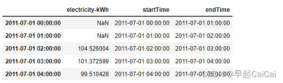
以上是每小时的用电量数据。数据被导出到一个Excel文件中。我们假设电表读数是在小时结束时记录的。
# Filter the data, keep the NaN and generate two excels, with and without NanhourlyElectricity.loc[abs(hourlyElectricity['electricity-kWh']) > 100000,'electricity-kWh'] = np.nantime = hourlyElectricity.index
index = ((time > np.datetime64('2012-07-26')) & (time < np.datetime64('2012-08-18'))) \| ((time > np.datetime64('2013-01-21')) & (time < np.datetime64('2013-03-08')))hourlyElectricity.loc[index,'electricity-kWh'] = np.nan
hourlyElectricityWithoutNaN = hourlyElectricity.dropna(axis=0, how='any')hourlyElectricity.to_excel('Data/hourlyElectricity.xlsx')
hourlyElectricityWithoutNaN.to_excel('Data/hourlyElectricityWithoutNaN.xlsx')
这段代码的功能是过滤数据,保留NaN,并分别生成两个Excel文件,一个包含NaN,一个不包含NaN。
具体来说:
- 首先,使用“loc”函数根据每小时用电量的绝对值是否大于100000来过滤数据,将超过该阈值的数据设置为NaN。
- 然后,创建一个名为“index”的布尔索引,根据时间戳选择数据,将指定时间范围内的数据设置为NaN。
- 接着,使用“dropna”函数删除任何包含NaN的行,并将结果存储在名为“hourlyElectricityWithoutNaN”的数据框中。
- 最后,使用“to_excel”函数将包含NaN的数据框“hourlyElectricity”和不包含NaN的数据框“hourlyElectricityWithoutNaN”分别导出到两个Excel文件中。
该代码的输出是两个Excel文件,分别为“hourlyElectricity.xlsx”和“hourlyElectricityWithoutNaN.xlsx”,用于进一步分析和处理数据。
plt.figure()
fig = hourlyElectricity.plot(fontsize = 15, figsize = (15, 6))
plt.tick_params(which=u'major', reset=False, axis = 'y', labelsize = 15)
fig.set_axis_bgcolor('w')
plt.title('All the hourly electricity data', fontsize = 16)
plt.ylabel('kWh')
plt.show()plt.figure()
fig = hourlyElectricity.iloc[26200:27400,:].plot(marker = 'o',label='hourly electricity', fontsize = 15, figsize = (15, 6))
plt.tick_params(which=u'major', reset=False, axis = 'y', labelsize = 15)
fig.set_axis_bgcolor('w')
plt.title('Hourly electricity data of selected days', fontsize = 16)
plt.ylabel('kWh')
plt.legend()
plt.show()


以上是每小时数据的图表。在第一个图表中,空缺的部分是由于电表故障时导致的数据缺失。在第二个图表中,您可以看到白天和晚上、工作日和周末之间的差异。
Derive daily consumption
计算每天消耗量
我们通过“reindex”成功获取了每日的电力消耗量。
dailyTimestamp = pd.date_range(start = '2011/7/1', end = '2014/10/31', freq = 'D')
electricityReindexed = electricity.reindex(dailyTimestamp, inplace = False)# Just in case, in order to use diff method, timestamp has to be in asending order.
electricityReindexed.sort_index(inplace = True)
dailyEnergy = electricityReindexed.diff(periods=1)['energy']dailyElectricity = pd.DataFrame(data = dailyEnergy.values, index = electricityReindexed.index - np.timedelta64(1,'D'), columns = ['electricity-kWh'])
dailyElectricity['startDay'] = dailyElectricity.index
dailyElectricity['endDay'] = dailyElectricity.index + np.timedelta64(1,'D')# Filter the data, keep the NaN and generate two excels, with and without NandailyElectricity.loc[abs(dailyElectricity['electricity-kWh']) > 2000000,'electricity-kWh'] = np.nantime = dailyElectricity.index
index = ((time > np.datetime64('2012-07-26')) & (time < np.datetime64('2012-08-18'))) | ((time > np.datetime64('2013-01-21')) & (time < np.datetime64('2013-03-08')))dailyElectricity.loc[index,'electricity-kWh'] = np.nan
dailyElectricityWithoutNaN = dailyElectricity.dropna(axis=0, how='any')dailyElectricity.to_excel('Data/dailyElectricity.xlsx')
dailyElectricityWithoutNaN.to_excel('Data/dailyElectricityWithoutNaN.xlsx')dailyElectricity.head()
代码解释:
-
dailyTimestamp = pd.date_range(start='2011/7/1', end='2014/10/31', freq='D'): 创建一个日期范围,从2011年7月1日到2014年10月31日,以每日为频率。 -
electricityReindexed = electricity.reindex(dailyTimestamp, inplace=False): 使用"reindex"方法将原始数据集重新索引为每日的时间戳,生成一个新的DataFrame对象。 -
electricityReindexed.sort_index(inplace=True): 确保时间戳按升序排序,以便后续使用"diff"方法。 -
dailyEnergy = electricityReindexed.diff(periods=1)['energy']: 使用"diff"方法计算每日能量消耗量的差异,并将结果存储在"dailyEnergy"列中。 -
dailyElectricity = pd.DataFrame(data=dailyEnergy.values, index=electricityReindexed.index - np.timedelta64(1, 'D'), columns=['electricity-kWh']): 创建一个新的DataFrame对象"dailyElectricity",其中包含每日电力消耗量和起始日期。 -
dailyElectricity['startDay'] = dailyElectricity.index: 添加一个"startDay"列,包含每日消耗量的起始日期。 -
dailyElectricity['endDay'] = dailyElectricity.index + np.timedelta64(1, 'D'): 添加一个"endDay"列,包含每日消耗量的结束日期。 -
dailyElectricity.loc[abs(dailyElectricity['electricity-kWh']) > 2000000, 'electricity-kWh'] = np.nan: 将电力消耗量超过2000000的值设为NaN(缺失值)。 -
time = dailyElectricity.index: 获取每日消耗量的时间索引。 -
index = ((time > np.datetime64('2012-07-26')) & (time < np.datetime64('2012-08-18'))) | ((time > np.datetime64('2013-01-21')) & (time < np.datetime64('2013-03-08'))): 创建一个布尔索引,用于筛选出指定时间范围内的数据。 -
dailyElectricity.loc[index, 'electricity-kWh'] = np.nan: 将指定时间范围内的电力消耗量设为NaN。 -
dailyElectricityWithoutNaN = dailyElectricity.dropna(axis=0, how='any'): 创建一个新的DataFrame对象"dailyElectricityWithoutNaN",删除包含NaN值的行。 -
dailyElectricity.to_excel('Data/dailyElectricity.xlsx'): 将"dailyElectricity"保存为Excel文件。 -
dailyElectricityWithoutNaN.to_excel('Data/dailyElectricityWithoutNaN.xlsx'): 将"dailyElectricityWithoutNaN"保存为Excel文件。 -
dailyElectricity.head(): 显示"dailyElectricity"的前几行数据。
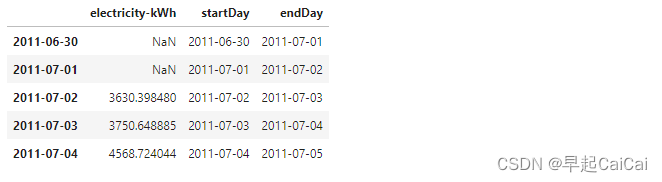
Above is the daily electricity consumption.
plt.figure()
fig = dailyElectricity.plot(figsize = (15, 6))
fig.set_axis_bgcolor('w')
plt.title('All the daily electricity data', fontsize = 16)
plt.ylabel('kWh')
plt.show()plt.figure()
fig = dailyElectricity.iloc[1000:1130,:].plot(marker = 'o', figsize = (15, 6))
fig.set_axis_bgcolor('w')
plt.title('Daily electricity data of selected days', fontsize = 16)
plt.ylabel('kWh')
plt.show()
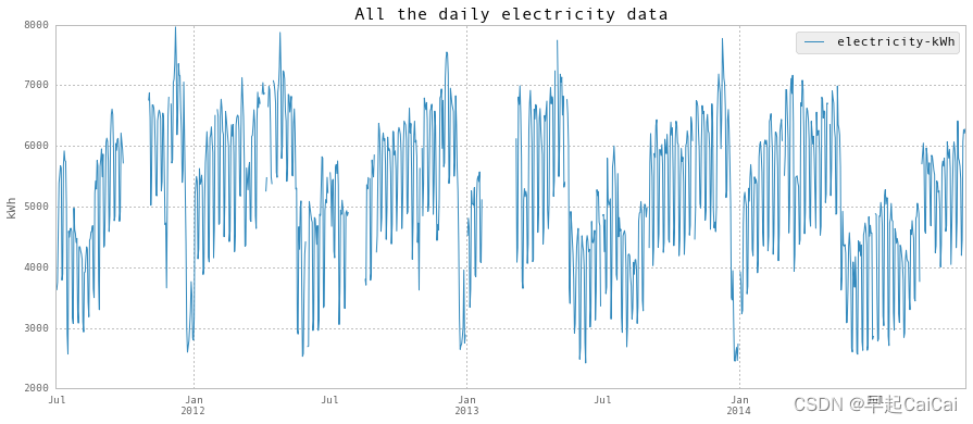
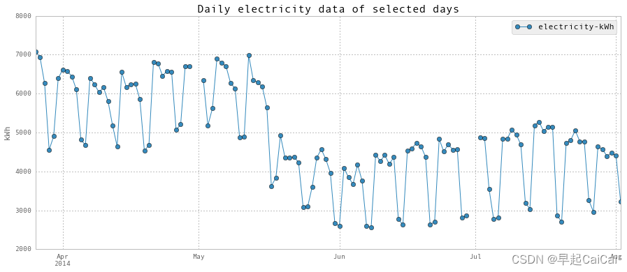
Above is the daily electricity plot.
超低的电力消耗发生在学期结束后,包括圣诞假期。此外,正如您在第二个图表中所看到的,夏季开始上学后能源消耗较低。
Chilled Water
冷水
We clean the chilled water data in the same way as electricity.
chilledWater = df[['Gund Main Energy - Ton-Days']]
chilledWater.head()
file = 'Data/monthly chilled water.csv'
monthlyChilledWaterFromFacility = pd.read_csv(file, header=0)
monthlyChilledWaterFromFacility.set_index(['month'], inplace = True)
monthlyChilledWaterFromFacility.head()
monthlyChilledWaterFromFacility['startDate'] = pd.to_datetime(monthlyChilledWaterFromFacility['startDate'], format="%m/%d/%y")
values = monthlyChilledWaterFromFacility.index.valueskeys = np.array(monthlyChilledWaterFromFacility['startDate'])dates = {}
for key, value in zip(keys, values):dates[key] = valuesortedDates =  np.sort(dates.keys())
sortedDates = sortedDates[sortedDates > np.datetime64('2011-11-01')]months = []
monthlyChilledWaterOrg = np.zeros((len(sortedDates) - 1))
for i in range(len(sortedDates) - 1):begin = sortedDates[i]end = sortedDates[i+1]months.append(dates[sortedDates[i]])monthlyChilledWaterOrg[i] = (np.round(chilledWater.loc[end,:] -  chilledWater.loc[begin,:], 1))monthlyChilledWater = pd.DataFrame(data = monthlyChilledWaterOrg, index = months, columns = ['chilledWater-TonDays'])fig,ax = plt.subplots(1, 1,figsize=(15,8))
#ax.set_axis_bgcolor('w')
#plt.plot(monthlyChilledWater, label='Our data processing from hourly data', marker = 'x', markersize = 15, linestyle = '')
plt.bar(np.arange(len(monthlyChilledWater))-0.5, monthlyChilledWater.values, label='Our data processing from hourly data')
plt.plot(monthlyChilledWaterFromFacility[5:-1]['chilledWater'],'or', label='Facility data')
plt.xticks(np.arange(0,len(months)),months)
plt.xlabel('Month',fontsize=15)
plt.ylabel('kWh',fontsize=15)
plt.xlim([0,len(months)])
plt.legend()
ax.set_xticklabels(months, rotation=40, fontsize=13)
plt.tick_params(which=u'major', reset=False, axis = 'y', labelsize = 15)
plt.title('Data Validation: comparison between our data processing and facilities',fontsize=20)text = 'Match! Our processing method is valid.'
ax.annotate(text, xy = (15, 2000), xytext = (5, 50), fontsize = 15, textcoords = 'offset points', ha = 'center', va = 'bottom')plt.show()
代码的解释如下:
首先,通过pd.to_datetime将monthlyChilledWaterFromFacility中的日期列转换为datetime格式。
然后,从monthlyChilledWaterFromFacility获取索引的值,并将其存储在values中。
接下来,将monthlyChilledWaterFromFacility中的开始日期列存储在keys中。
通过循环遍历keys和values,将日期和索引值存储在dates字典中。
对dates字典的键进行排序,并将排序后的日期存储在sortedDates中。然后,从sortedDates中筛选出大于指定日期的日期。
创建空列表months,用于存储月份。
使用np.zeros创建一个长度为sortedDates减1的零数组monthlyChilledWaterOrg。
通过循环遍历sortedDates,计算每个月的冷水消耗量,并将结果存储在monthlyChilledWaterOrg中。
将monthlyChilledWaterOrg转换为DataFrame,使用months作为索引,列名为chilledWater-TonDays。
创建一个图表,并使用plt.bar绘制我们从小时数据处理得到的冷水消耗量,使用plt.plot绘制设备数据。
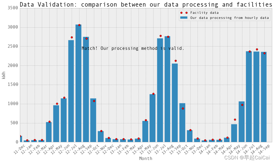
上图中红点为设施的数据,bar为我们从每小时数据获取的每天的数据,两者基本一致,说明我们处理的方法是正确的
hourlyTimestamp = pd.date_range(start = '2011/7/1', end = '2014/10/31', freq = 'H')
chilledWater.reindex(hourlyTimestamp, inplace = True)# Just in case, in order to use diff method, timestamp has to be in asending order.
chilledWater.sort_index(inplace = True)
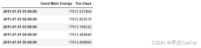
hourlyEnergy = chilledWater.diff(periods=1)hourlyChilledWater = pd.DataFrame(data = hourlyEnergy.values, index = hourlyEnergy.index, columns = ['chilledWater-TonDays'])
hourlyChilledWater['startTime'] = hourlyChilledWater.index
hourlyChilledWater['endTime'] = hourlyChilledWater.index + np.timedelta64(1,'h')hourlyChilledWater.loc[abs(hourlyChilledWater['chilledWater-TonDays']) > 50,'chilledWater-TonDays'] = np.nanhourlyChilledWaterWithoutNaN = hourlyChilledWater.dropna(axis=0, how='any')hourlyChilledWater.to_excel('Data/hourlyChilledWater.xlsx')
hourlyChilledWaterWithoutNaN.to_excel('Data/hourlyChilledWaterWithoutNaN.xlsx')plt.figure()
fig = hourlyChilledWater.plot(fontsize = 15, figsize = (15, 6))
plt.tick_params(which=u'major', reset=False, axis = 'y', labelsize = 15)
fig.set_axis_bgcolor('w')
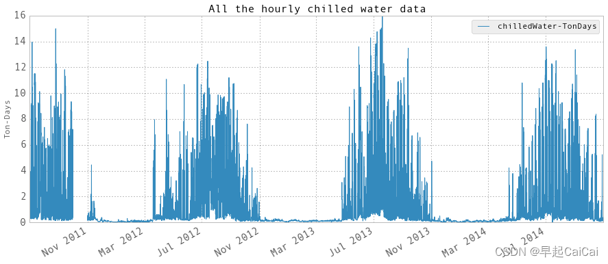
plt.title('All the hourly chilled water data', fontsize = 16)
plt.ylabel('Ton-Days')
plt.show()hourlyChilledWater.head()
代码的解释如下:
首先,使用pd.date_range生成从开始日期到结束日期的逐小时时间戳,存储在hourlyTimestamp中。
通过reindex方法,将冷水数据重新索引为逐小时时间戳,并将结果存储在chilledWater中。
接下来,对chilledWater进行按索引排序,以确保时间戳按升序排列。
使用diff方法计算每小时的冷水消耗量,并将结果存储在hourlyEnergy中。
创建一个DataFrame,使用hourlyEnergy的值作为数据,时间戳作为索引,列名为chilledWater-TonDays。
添加startTime和endTime列,分别表示每小时的起始时间和结束时间。
通过loc方法,将冷水消耗量绝对值大于50的数据设置为NaN。
使用dropna方法删除含有NaN值的行,并将结果存储在hourlyChilledWaterWithoutNaN中。
将hourlyChilledWater和hourlyChilledWaterWithoutNaN分别保存为Excel文件。
创建一个图表,并使用plot方法绘制所有小时级冷水数据。
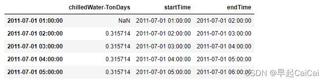
上图为
hourlyEnergy的值
dailyTimestamp = pd.date_range(start = '2011/7/1', end = '2014/10/31', freq = 'D')
chilledWaterReindexed = chilledWater.reindex(dailyTimestamp, inplace = False)chilledWaterReindexed.sort_index(inplace = True)
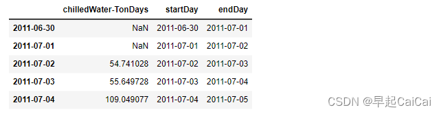
dailyEnergy = chilledWaterReindexed.diff(periods=1)['Gund Main Energy - Ton-Days']dailyChilledWater = pd.DataFrame(data = dailyEnergy.values, index = chilledWaterReindexed.index - np.timedelta64(1,'D'), columns = ['chilledWater-TonDays'])
dailyChilledWater['startDay'] = dailyChilledWater.index
dailyChilledWater['endDay'] = dailyChilledWater.index + np.timedelta64(1,'D')dailyChilledWaterWithoutNaN = dailyChilledWater.dropna(axis=0, how='any')dailyChilledWater.to_excel('Data/dailyChilledWater.xlsx')
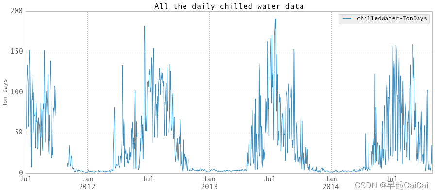
dailyChilledWaterWithoutNaN.to_excel('Data/dailyChilledWaterWithoutNaN.xlsx')plt.figure()
fig = dailyChilledWater.plot(fontsize = 15, figsize = (15, 6))
plt.tick_params(which=u'major', reset=False, axis = 'y', labelsize = 15)
fig.set_axis_bgcolor('w')
plt.title('All the daily chilled water data', fontsize = 16)
plt.ylabel('Ton-Days')
plt.show()dailyChilledWater.head()
代码的解释如下:
首先,使用pd.date_range生成从开始日期到结束日期的逐日时间戳,存储在dailyTimestamp中。
通过reindex方法,将冷水数据重新索引为逐日时间戳,并将结果存储在chilledWaterReindexed中。
接下来,对chilledWaterReindexed进行按索引排序,以确保时间戳按升序排列。
使用diff方法计算每天的冷水消耗量,并将结果存储在dailyEnergy中,列名为’Gund Main Energy - Ton-Days’。
创建一个DataFrame,使用dailyEnergy的值作为数据,时间戳减去1天作为索引,列名为chilledWater-TonDays。
添加startDay和endDay列,分别表示每天的起始时间和结束时间。
使用dropna方法删除含有NaN值的行,并将结果存储在dailyChilledWaterWithoutNaN中。
将dailyChilledWater和dailyChilledWaterWithoutNaN分别保存为Excel文件。
创建一个图表,并使用plot方法绘制所有每日级冷水数据。
Steam
蒸汽
steam = df[['Gund Condensate FlowTotal - LBS']]
steam.head()

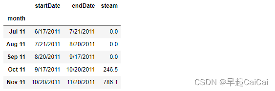
file = 'Data/monthly steam.csv'
monthlySteamFromFacility = pd.read_csv(file, header=0)
monthlySteamFromFacility.set_index(['month'], inplace = True)
monthlySteamFromFacility.head()
monthlySteamFromFacility['startDate'] = pd.to_datetime(monthlySteamFromFacility['startDate'], format="%m/%d/%Y")
values = monthlySteamFromFacility.index.valueskeys = np.array(monthlySteamFromFacility['startDate'])dates = {}
for key, value in zip(keys, values):dates[key] = valuesortedDates =  np.sort(dates.keys())
sortedDates = sortedDates[sortedDates > np.datetime64('2011-11-01')]months = []
monthlySteamOrg = np.zeros((len(sortedDates) - 1))
for i in range(len(sortedDates) - 1):begin = sortedDates[i]end = sortedDates[i+1]months.append(dates[sortedDates[i]])monthlySteamOrg[i] = (np.round(steam.loc[end,:] -  steam.loc[begin,:], 1))monthlySteam = pd.DataFrame(data = monthlySteamOrg, index = months, columns = ['steam-LBS'])# 867 LBS ~= 1MMBTU steamfig,ax = plt.subplots(1, 1,figsize=(15,8))
#ax.set_axis_bgcolor('w')
#plt.plot(monthlySteam/867, label='Our data processing from hourly data')
plt.bar(np.arange(len(monthlySteam))-0.5, monthlySteam.values/867, label='Our data processing from hourly data')
plt.plot(monthlySteamFromFacility.loc[months,'steam'],'or', label='Facility data')
plt.xticks(np.arange(0,len(months)),months)
plt.xlabel('Month',fontsize=15)
plt.ylabel('Steam (MMBTU)',fontsize=15)
plt.xlim([0,len(months)])
plt.legend()
ax.set_xticklabels(months, rotation=40, fontsize=13)
plt.tick_params(which=u'major', reset=False, axis = 'y', labelsize = 15)
plt.title('Comparison between our data processing and facilities - Steam',fontsize=20)text = 'Match! Our processing method is valid.'
ax.annotate(text, xy = (9, 1500), xytext = (5, 50), fontsize = 15, textcoords = 'offset points', ha = 'center', va = 'bottom')plt.show()
代码的解释如下:
首先,将monthlySteamFromFacility中的"startDate"列转换为日期时间格式,格式为"%m/%d/%Y",并将结果存储在该列中。
将monthlySteamFromFacility的索引值存储在values中。
创建一个keys数组,其中存储了monthlySteamFromFacility的"startDate"列的值。
创建一个空字典dates,用于存储"startDate"和索引值之间的映射关系。
使用zip函数将keys和values进行迭代,将"startDate"和索引值存储在dates字典中。
对dates.keys()进行排序,将结果存储在sortedDates中。
从sortedDates中选择大于日期'2011-11-01'的日期,并重新赋值给sortedDates。
创建一个空列表months,用于存储每个时间段的月份。
创建一个长度为len(sortedDates) - 1的零数组monthlySteamOrg。
使用循环遍历sortedDates中的日期,并根据日期计算每个时间段的蒸汽消耗量。
将对应的月份添加到months列表中。
将计算得到的蒸汽消耗量存储在monthlySteamOrg数组中。
创建一个DataFrame,使用monthlySteamOrg的值作为数据,months作为索引,列名为"steam-LBS"。
创建一个图表,并使用bar和plot方法分别绘制我们的数据处理结果和设施数据的对比。
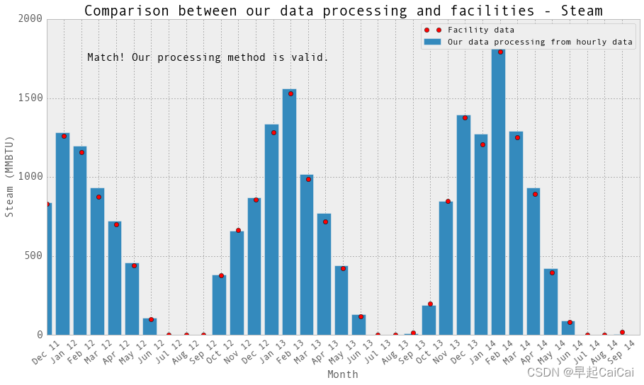
我们的处理数据与设备的数据是一致的
和上面一样:绘制出 hourly steam data; daily steam data
hourlyTimestamp = pd.date_range(start = '2011/7/1', end = '2014/10/31', freq = 'H')
steam.reindex(hourlyTimestamp, inplace = True)# Just in case, in order to use diff method, timestamp has to be in asending order.
steam.sort_index(inplace = True)
hourlyEnergy = steam.diff(periods=1)hourlySteam = pd.DataFrame(data = hourlyEnergy.values, index = hourlyEnergy.index, columns = ['steam-LBS'])
hourlySteam['startTime'] = hourlySteam.index
hourlySteam['endTime'] = hourlySteam.index + np.timedelta64(1,'h')hourlySteam.loc[abs(hourlySteam['steam-LBS']) > 100000,'steam-LBS'] = np.nanplt.figure()
fig = hourlySteam.plot(fontsize = 15, figsize = (15, 6))
plt.tick_params(which=u'major', reset=False, axis = 'y', labelsize = 17)
fig.set_axis_bgcolor('w')
plt.title('All the hourly steam data', fontsize = 16)
plt.ylabel('LBS')
plt.show()hourlySteamWithoutNaN = hourlySteam.dropna(axis=0, how='any')hourlySteam.to_excel('Data/hourlySteam.xlsx')
hourlySteamWithoutNaN.to_excel('Data/hourlySteamWithoutNaN.xlsx')hourlySteam.head()
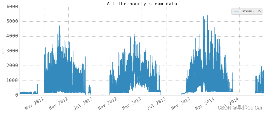
hourly steam data
dailyTimestamp = pd.date_range(start = '2011/7/1', end = '2014/10/31', freq = 'D')
steamReindexed = steam.reindex(dailyTimestamp, inplace = False)steamReindexed.sort_index(inplace = True)
dailyEnergy = steamReindexed.diff(periods=1)['Gund Condensate FlowTotal - LBS']dailySteam = pd.DataFrame(data = dailyEnergy.values, index = steamReindexed.index - np.timedelta64(1,'D'), columns = ['steam-LBS'])
dailySteam['startDay'] = dailySteam.index
dailySteam['endDay'] = dailySteam.index + np.timedelta64(1,'D')plt.figure()
fig = dailySteam.plot(fontsize = 15, figsize = (15, 6))
plt.tick_params(which=u'major', reset=False, axis = 'y', labelsize = 15)
fig.set_axis_bgcolor('w')
plt.title('All the daily steam data', fontsize = 16)
plt.ylabel('LBS')
plt.show()dailySteamWithoutNaN = dailyChilledWater.dropna(axis=0, how='any')dailySteam.to_excel('Data/dailySteam.xlsx')
dailySteamWithoutNaN.to_excel('Data/dailySteamWithoutNaN.xlsx')dailySteam.head()
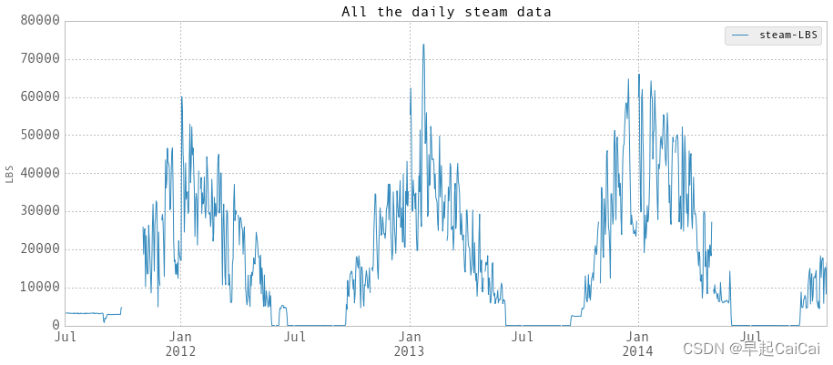
daily steam data
Reference
cs109-energy+哈佛大学能源探索项目 Part-1(项目背景)
一个完整的机器学习项目实战代码+数据分析过程:哈佛大学能耗预测项目
Part 1-3 Project Overview, Data Wrangling and Exploratory Analysis-DEC10
Prediction of Buildings Energy Consumption
相关文章:
cs109-energy+哈佛大学能源探索项目 Part-2.1(Data Wrangling)
博主前期相关的博客见下: cs109-energy哈佛大学能源探索项目 Part-1(项目背景) 这次主要讲数据的整理。 Data Wrangling 数据整理 在哈佛的一些大型建筑中,有三种类型的能源消耗,电力,冷冻水和蒸汽。 冷冻…...
__101对称二叉树------进阶:你可以运用递归和迭代两种方法解决这个问题吗?---本题还没用【迭代】去实现
101对称二叉树 原题链接:完成情况:解题思路:参考代码: 原题链接: 101. 对称二叉树 https://leetcode.cn/problems/symmetric-tree/ 完成情况: 解题思路: 递归的难点在于:找到可以…...
怎么取消只读模式?硬盘进入只读模式怎么办?
案例:电脑磁盘数据不能修改怎么办? 【今天工作的时候,我想把最近的更新的资料同步到电脑上的工作磁盘,但是发现我无法进行此操作,也不能对磁盘里的数据进行改动。有没有小伙伴知道这是怎么一回事?】 在使…...

如何使用Java生成Web项目验证码
使用Java编写Web项目验证码 验证码是Web开发中常用的一种验证方式,可以防止机器恶意攻击。本文将介绍如何使用Java编写Web项目验证码,包括步骤、示例和测试。 步骤 1. 添加依赖 首先需要在项目中添加以下依赖: <dependency><groupId>com.google.code.kaptc…...

【读书笔记】《亲密关系》
作者:美国的罗兰米勒 刚拿到这本书的时候,就被最后将近100页的参考文献折服了,让我认为这本书极具专业性。 作者使用了14章,从人与人之间是如何相互吸引的,讲到如何相处与沟通,后又讲到如何面对冲突与解决矛…...

面试季,真的太狠了...
金三银四面试季的复盘,真的太狠了… 面试感受 先说一个字 是真的 “ 累 ” 安排的太满的后果可能就是一天只吃一顿饭,一直奔波在路上 不扯这个了,给大家说说面试吧,我工作大概两年多的时间,大家可以参考下 在整个面…...

2023年十大最佳黑客工具!
用心做分享,只为给您最好的学习教程 如果您觉得文章不错,欢迎持续学习 在今年根据实际情况,结合全球黑客共同推崇,选出了2023年十大最佳黑客工具。 每一年,我都会持续更新,并根据实际现实情况随时更改…...

每日练习---C语言
目录 前言: 1.打印菱形 1.1补充练习 2.打印水仙花 2.1补充训练 前言: 记录博主做题的收获,以及提升自己的代码能力,今天写的题目是:打印菱形、打印水仙花数。 1.打印菱形 我们先看到牛客网的题:OJ链…...

边缘计算如何推动物联网的发展
随着物联网(IoT)的快速发展,物联网设备数量呈现爆炸性增长,这给网络带来了巨大的压力和挑战。边缘计算作为一种新兴的计算模式,旨在解决数据处理和通信在网络传输中的延迟和带宽限制问题,从而提高数据处理效…...

第五章 栈与队列
目录 一、用栈实现队列二、用队列实现栈三、有效的括号四、删除字符串中的所有相邻重复项五、逆波兰表达式求值六、滑动窗口最大值七、前 K 个高频元素 一、用栈实现队列 Leetcode 232 class MyQueue { public:stack<int> in, out;MyQueue() {}void push(int x) {in.pu…...

PyQt5桌面应用开发(16):定制化控件-QPainter绘图
本文目录 PyQt5桌面应用系列画画图,喝喝茶QPainter和QPixmapQPixmapQPainter绘制事件 一个魔改的QLabelCanvas类主窗口主程序: 总结 PyQt5桌面应用系列 PyQt5桌面应用开发(1):需求分析 PyQt5桌面应用开发(2…...
spring5源码篇(9)——mybatis-spring整合原理
spring-framework 版本:v5.3.19 spring和mybatis的整合无非主要就是以下几个方面: 1、SqlSessionFactory怎么注入? 2、Mapper代理怎么注入? 3、为什么要接管mybatis事务? 文章目录 一、SqlSessionFactory怎么注入SqlSe…...

为什么需要防雷接地,防雷接地的作用是什么
为什么需要电气接地? 您是否曾经在工作条件下使用任何电器时接触过电击?几乎每个人的答案都是肯定的,有时这些电击是轻微的,但有时会对电气和电子设备造成损坏,并可能危及生命。为防止对人的生命和电器造成任何损害&a…...
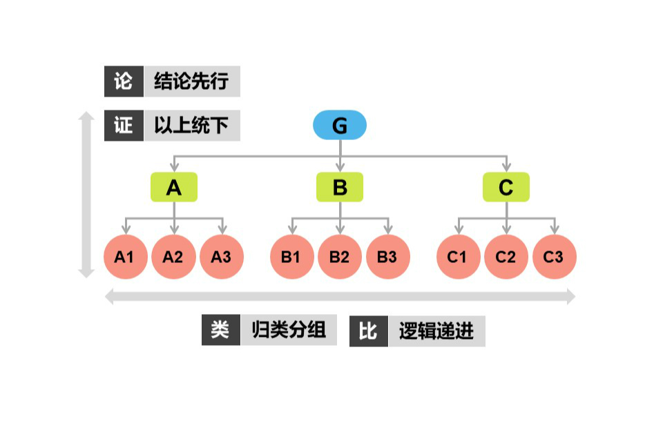
如何应用金字塔模型提高结构化表达能力
看一下结构化表达的定义: 结构化表达:是基于结构化思维,理清事物整理与部分之间关系、换位思考后,进行简洁、清晰和有信服力的表达,是一种让受众听得明白、记得清楚、产生认同的精益沟通方式。 结构化表达的基本原则是…...

2023年系统分析师考前几页纸
企业战略规划是用机会和威胁评价现在和未来的环境,用优势和劣势评价企业现状,进而选择和确定企业的总体和长远目标,制定和抉择实现目标的行动方案。信息系统战略规划关注的是如何通过该信息系统来支撑业务流程的运作,进而实现企业的关键业务目标,其重点在于对信息系统远景…...
openwrt-安装NGINX
openwrt-安装NGINX 介绍 OpenWrt 是一个用于嵌入式设备的开源操作系统。它基于 Linux 内核,并且主要被设计用于路由器和网络设备。 OpenWrt 的主要特点包括: 完全可定制:OpenWrt 提供了一个完全可写的文件系统,用户可以自定义设…...

Linux安装MongoDB数据库并内网穿透在外远程访问
文章目录 前言1.配置Mongodb源2.安装MongoDB数据库3.局域网连接测试4.安装cpolar内网穿透5.配置公网访问地址6.公网远程连接7.固定连接公网地址8.使用固定公网地址连接 转发自CSDN cpolarlisa的文章:Linux服务器安装部署MongoDB数据库 - 无公网IP远程连接「内网穿透…...

flutter系列之:使用AnimationController来控制动画效果
文章目录 简介构建一个要动画的widget让图像动起来总结 简介 之前我们提到了flutter提供了比较简单好用的AnimatedContainer和SlideTransition来进行一些简单的动画效果,但是要完全实现自定义的复杂的动画效果,还是要使用AnimationController。 今天我…...

golang 函数调用栈笔记
一个被函数在栈上的情况:(栈从高地址向低地址延伸) 返回地址(函数执行结束后,会跳转到这个地址执行) BP(函数的栈基)局部变量返回值(指的是函数返回值,eg&am…...

云端一体助力体验升级和业务创新
随着音视频和AI技术的发展,在满足用户基础体验和需求情况下,更极致的用户体验和更丰富的互动玩法,成为各个平台打造核心竞争力的关键。LiveVideoStackCon 2022 北京站邀请到火山引擎视频云华南区业务负责人——张培垒,基于节跳动音…...

高性能Windows流媒体服务器部署:5大核心技术与3种实战架构深度解析
高性能Windows流媒体服务器部署:5大核心技术与3种实战架构深度解析 【免费下载链接】srs-windows 项目地址: https://gitcode.com/gh_mirrors/sr/srs-windows 在Windows平台上构建专业级流媒体服务系统,需要综合考虑协议兼容性、性能优化和部署架…...

Wechat2RSS:微信公众号转RSS订阅工具
文章目录Wechat2RSS:微信公众号转RSS订阅工具Wechat2RSS:微信公众号转RSS订阅工具 ttttmr开源的Wechat2RSS项目,目前在GitHub上获得1409颗Star,项目地址为https://github.com/ttttmr/Wechat2RSS。该工具的核心作用是将微信公众号…...
)
别再用SonarQube凑数了!DeepSeek原生圈复杂度引擎的6大颠覆性能力(含GitHub私有部署密钥)
更多请点击: https://kaifayun.com 第一章:DeepSeek圈复杂度分析的底层原理与范式革命 DeepSeek圈复杂度分析并非传统McCabe度量的简单复刻,而是基于控制流图(CFG)动态重构与语义感知路径裁剪的双重机制构建的新范式。…...

FM3773 低功耗离线式恒流/恒压 PSR 控制器
概述 FM3773 是一种高性能的交流/直流用于电池充电器和适配器的电源控制器,内置 850V 功率三极管。该设备采用脉冲频率调制(PFM)的方法来建立非连续导通模式(DCM)反激式电源。 FM3773 提供精确的恒定电压,恒…...

Linux服务器被挖矿木马劫持的五步应急处置指南
1. 这不是“中病毒”,是服务器被劫持成了矿机——先别慌,但必须立刻断网“服务器被黑客攻击,用来挖矿!”——这句话在运维圈里一出,比收到OOM告警还让人头皮发紧。它不像网页被挂马、数据库被拖库那样有明显业务影响&a…...

DAIR-V2X-V数据集深度评测:与KITTI、nuScenes比,它到底强在哪?
DAIR-V2X-V数据集深度评测:与KITTI、nuScenes比,它到底强在哪? 当技术团队着手开发面向中国道路的自动驾驶系统时,数据集的选择往往成为第一个关键决策点。过去十年间,KITTI和nuScenes等国际数据集一直是行业标杆&…...

如何用Nucleus Co-Op让单机游戏变身本地多人分屏神器
如何用Nucleus Co-Op让单机游戏变身本地多人分屏神器 【免费下载链接】nucleuscoop Starts multiple instances of a game for split-screen multiplayer gaming! 项目地址: https://gitcode.com/gh_mirrors/nu/nucleuscoop 还在为想和朋友一起玩游戏却只有一台电脑而烦…...

智能体任务分配算法:从启发式到深度强化学习的演进与实践
1. 项目概述:从“谁来做”到“如何做得更好”的智能进化在机器人集群、无人机编队或是自动化仓储系统中,我们常常面临一个看似简单实则复杂的问题:眼前有一堆任务,手头有一群可用的智能体(机器人、无人机、服务器等&am…...

动物森友会岛屿设计终极指南:用Happy Island Designer打造梦想岛屿
动物森友会岛屿设计终极指南:用Happy Island Designer打造梦想岛屿 【免费下载链接】HappyIslandDesigner "Happy Island Designer (Alpha)",是一个在线工具,它允许用户设计和定制自己的岛屿。这个工具是受游戏《动物森友会》(Anim…...

Hyper-V离散设备分配图形化解决方案:企业级虚拟化性能优化实践
Hyper-V离散设备分配图形化解决方案:企业级虚拟化性能优化实践 【免费下载链接】DDA 实现Hyper-V离散设备分配功能的图形界面工具。A GUI Tool For Hyper-Vs Discrete Device Assignment(DDA). 项目地址: https://gitcode.com/gh_mirrors/dd/DDA 在数字化转…...