【无线传感器】使用 MATLAB和 XBee连续监控温度传感器无线网络研究(Matlab代码实现)
💥💥💞💞欢迎来到本博客❤️❤️💥💥
🏆博主优势:🌞🌞🌞博客内容尽量做到思维缜密,逻辑清晰,为了方便读者。
⛳️座右铭:行百里者,半于九十。
📋📋📋本文目录如下:🎁🎁🎁
目录
💥1 概述
📚2 运行结果
🎉3 参考文献
🌈4 Matlab代码及数据

💥1 概述
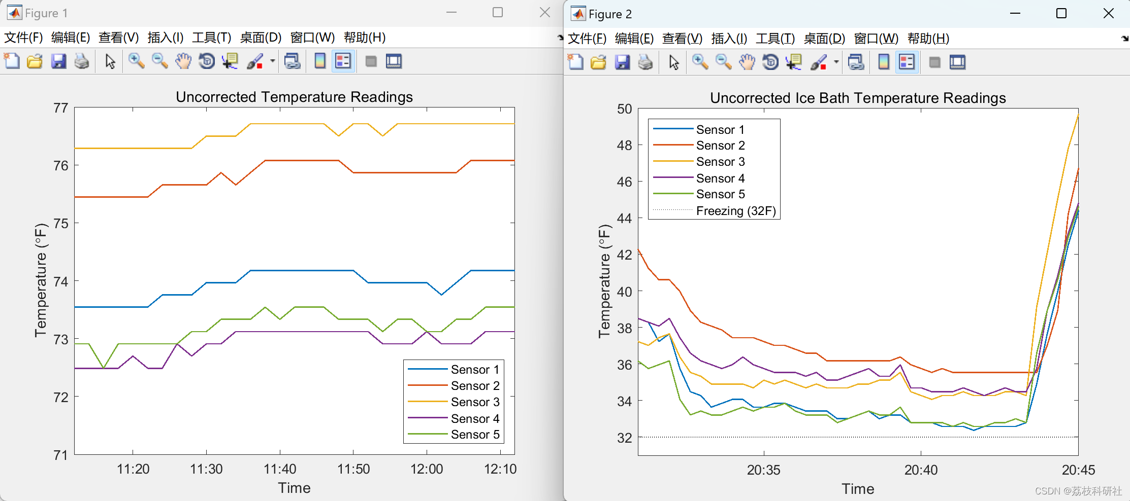
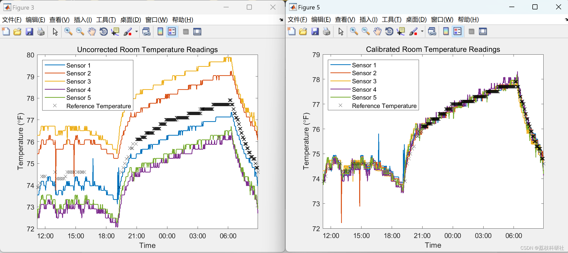
在本文中,MATLAB 用于通过与使用 XBee 系列 2 模块构建的温度传感器无线网络进行交互,连续监控整个公寓的温度。每个XBee边缘节点从多个温度传感器读取模拟电压(与温度成线性比例)。读数通过协调器XBee模块传输回MATLAB。本文说明了如何操作、获取和分析来自连接到多个 XBee 边缘节点的多个传感器网络的数据。数据采集时间从数小时到数天不等,以帮助设计和构建智能恒温器系统。
📚2 运行结果

 部分代码:
部分代码:
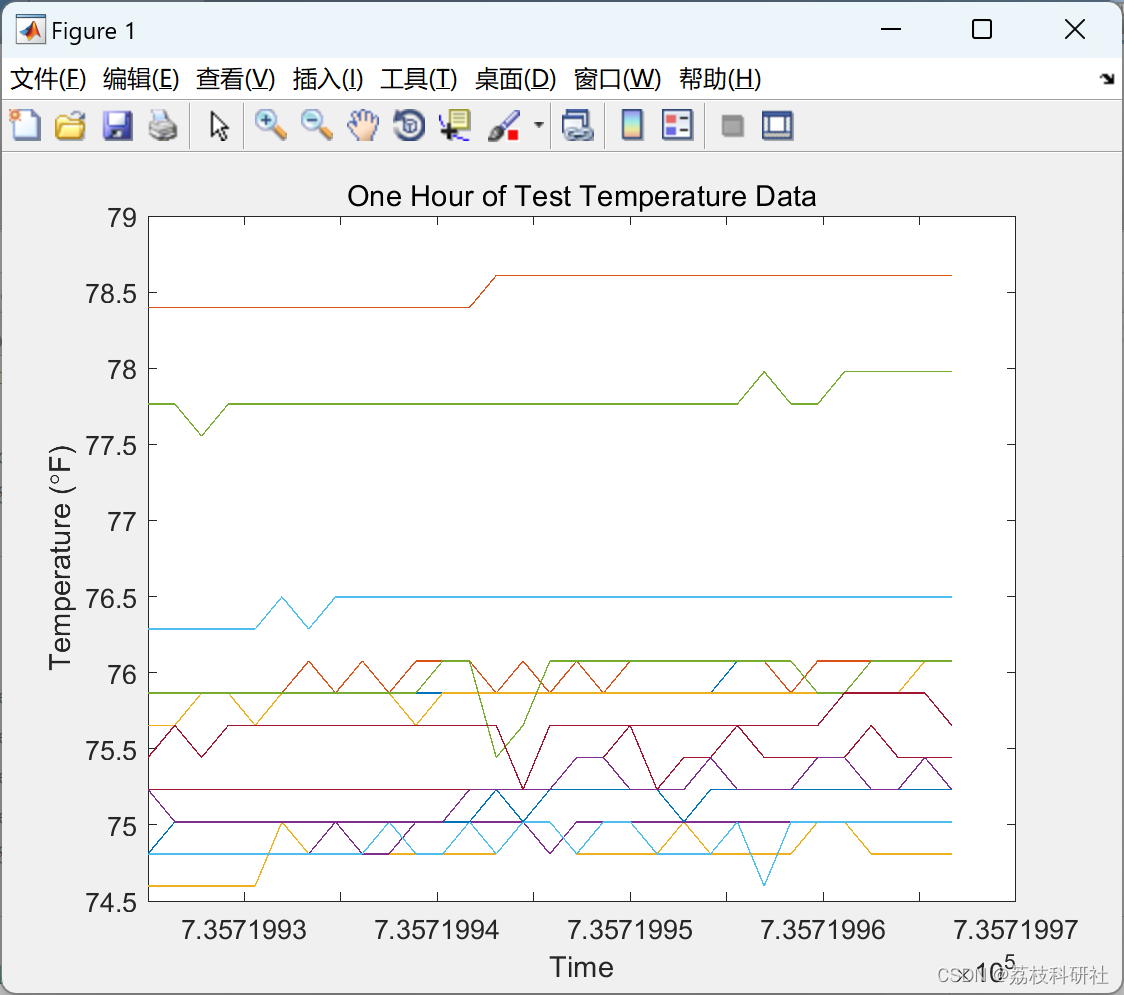
%% Overview of Data
% As I mentioned in a previous post, I collected the temperature every two
% minutes over the course of 9 days. I placed 14 sensors in my apartment: 9
% located inside, 2 located outside, and 3 located in radiators. The data
% is stored in the file <../twoweekstemplog.txt |twoweekstemplog.txt|>.
[tempF,ts,location,lineSpecs] = XBeeReadLog('twoweekstemplog.txt',60);
tempF = calibrateTemperatures(tempF);
plotTemps(ts,tempF,location,lineSpecs)
legend('off')
xlabel('Date')
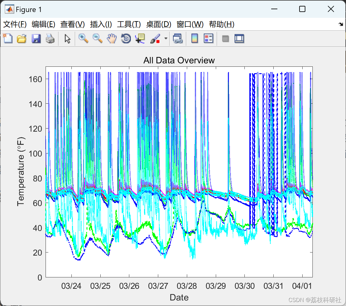
title('All Data Overview')
%%
% _Figure 1: All temperature data from a 9 day period._
%
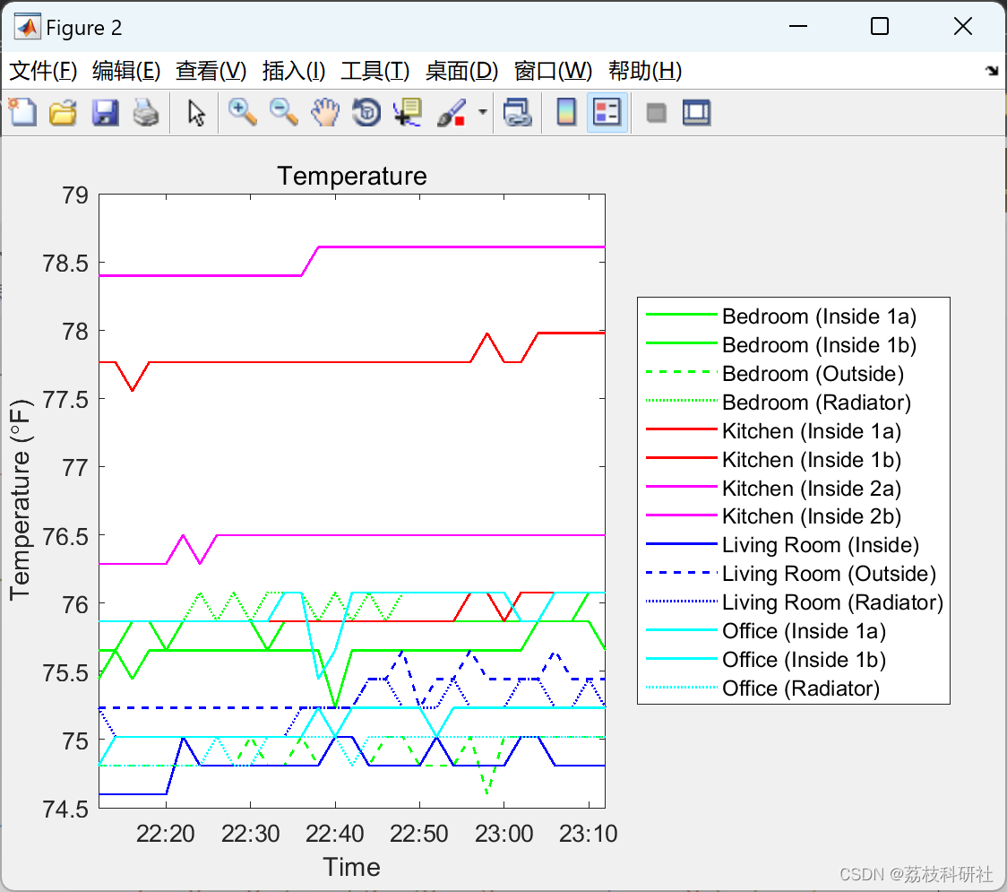
% That graph is a bit too cluttered to be very meaningful. Let me remove
% the radiator data and the legend and see if that helps.
notradiator = [1 2 3 5 6 7 8 9 10 12 13];
plotTemps(ts,tempF(:,notradiator),location(notradiator),lineSpecs(notradiator,:))
legend('off')
xlabel('Date')
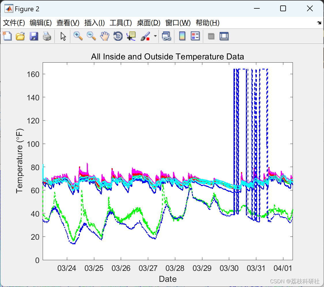
title('All Inside and Outside Temperature Data')
%%
% _Figure 2: Just inside and outside temperature data, with radiator data removed._
%
% Now I can see some places where one of the outdoor temperature sensors
% (blue line) gave erroneous data, so let's remove those data points. This
% data was collected in March in Massachusetts, so I can safely assume the
% outdoor temperature never reached 80 F. I replaced any values above 80 F
% with |NaN| (not-a-number) so they are ignored in further analysis.
outside = [3 10];
outsideTemps = tempF(:,outside);
toohot = outsideTemps>80;
outsideTemps(toohot) = NaN;
tempF(:,outside) = outsideTemps;
plotTemps(ts,tempF(:,notradiator),location(notradiator),lineSpecs(notradiator,:))
legend('off')
xlabel('Date')
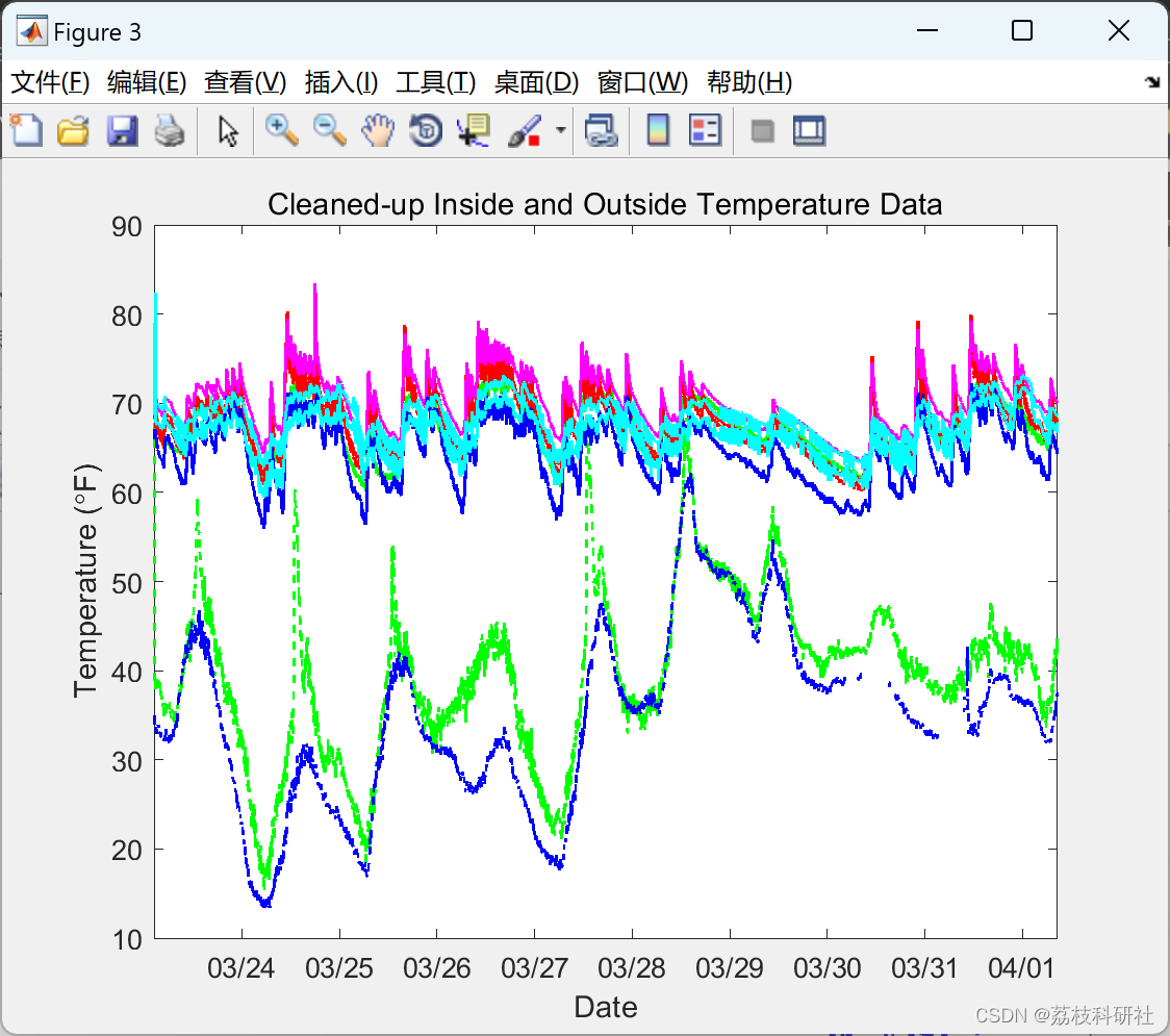
title('Cleaned-up Inside and Outside Temperature Data')
%%
% _Figure 3: Inside and outside temperature data with erroneous data removed._
%
% I'll also remove all but one inside sensor per room, and give the
% remaining sensors shorter names, to keep the graph from getting too
% cluttered.
show = [1 5 9 12 10 3];
location(show) = ...
{'Bedroom','Kitchen','Living Room','Office','Front Porch','Side Yard'}';
plotTemps(ts,tempF(:,show),location(show),lineSpecs(show,:))
ylim([0 90])
legend('Location','SouthEast')
xlabel('Date')
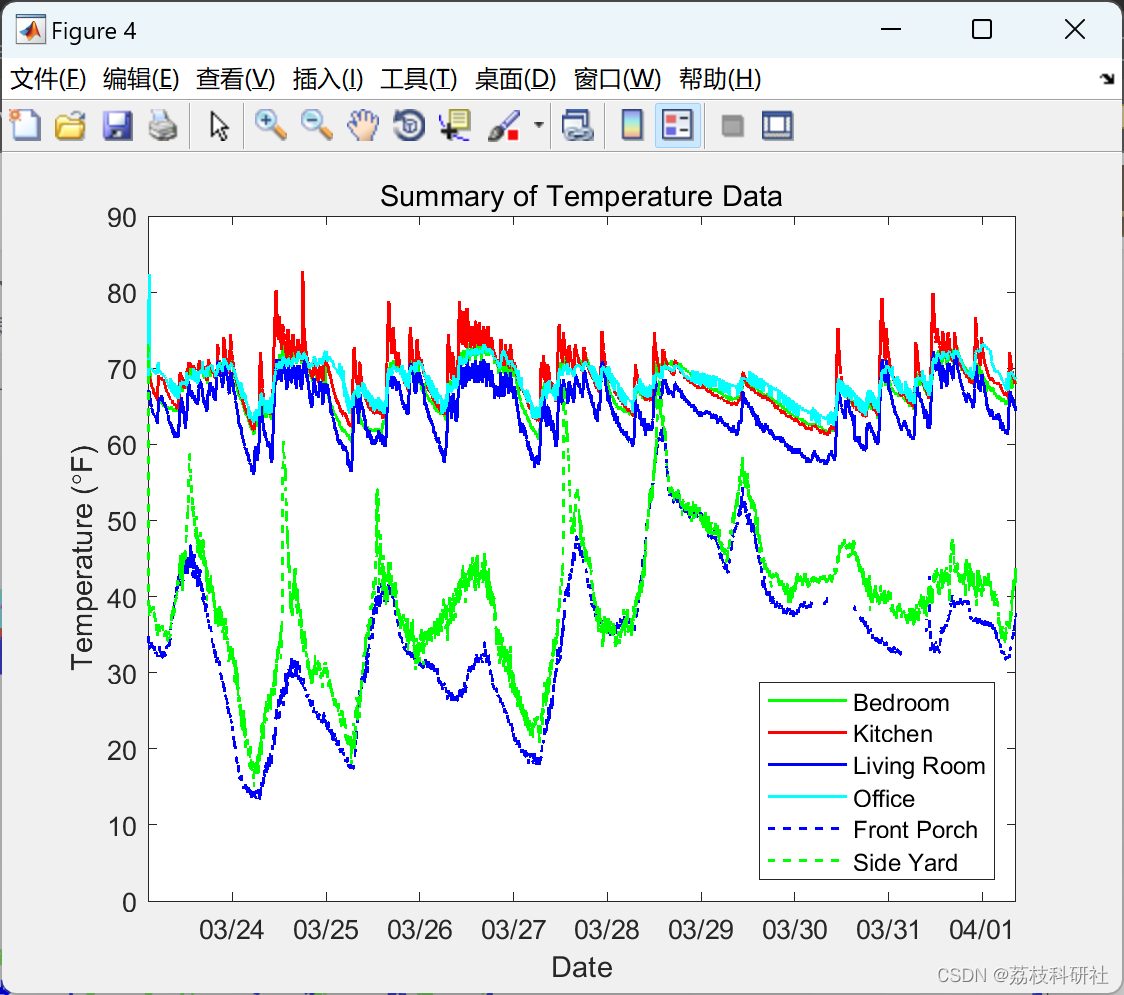
title('Summary of Temperature Data')
%%
% _Figure 4: Summary of temperature data with only one inside temperature
% sensor per room with outside temperatures._
%
% That looks much better. This data was collected over the course of 9
% days, and the first thing that stands out to me is the periodic outdoor
% temperature, which peaks every day at around noon. I also notice a sharp
% spike in the side yard (green) temperature on most days. My front porch
% (blue) is located on the north side of my apartment, and does not get
% much sun. My side yard is on the east side of my apartment, and that
% spike probably corresponds to when the sun hits the sensor from between
% my apartment and the building next door.
%% When do my radiators start to heat up?
% The radiator temperature can be used to measure how long it takes for my
% boiler and radiators to warm up after the heat has been turned on. Let's
% take a look at 1 day of data from the living room radiator:
% Grab the Living Room Radiator Temperature (index 11) from the |tempF| matrix.
radiatorTemp = tempF(:,11);
% Fill in any missing values:
validts = ts(~isnan(radiatorTemp));
validtemp = radiatorTemp(~isnan(radiatorTemp));
nants = ts(isnan(radiatorTemp));
radiatorTemp(isnan(radiatorTemp)) = interp1(validts,validtemp,nants);
% Plot the data
oneday = [ts(1) ts(1)+1];
figure
plot(ts,radiatorTemp,'k.-')
xlim(oneday)
xlabel('Time')
ylabel('Radiator Temperature (\circF)')
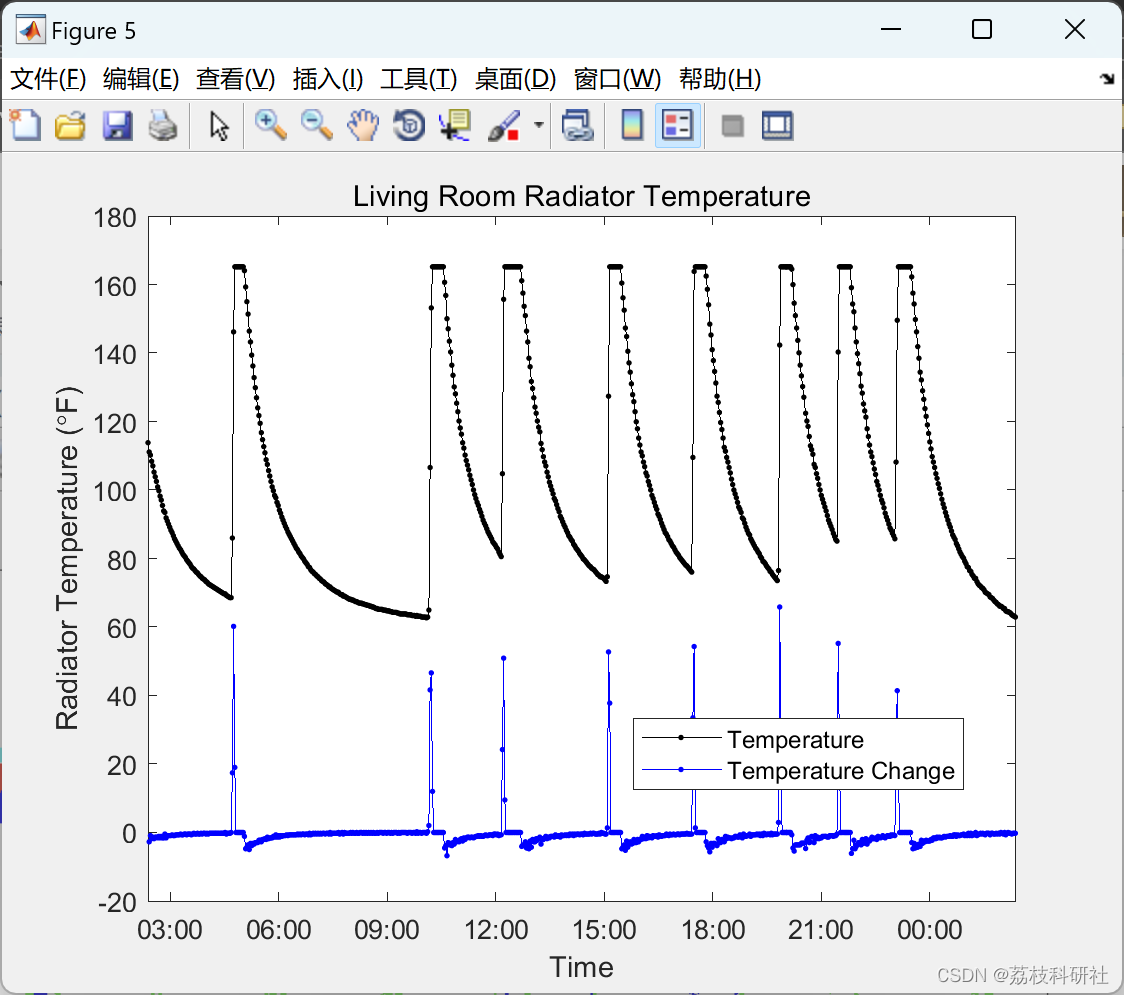
title('Living Room Radiator Temperature')
datetick('keeplimits')
snapnow
%%
% _Figure 5: One day of temperature data from the living room radiator._
%
% As expected, I see a sharp rise in the radiator temperature, followed by
% a short leveling off (when the radiator temperature maxes out the
% temperature sensor), and finally a gradual cooling of the radiator. Let
% me superimpose the rate of change in temperature onto the plot.
tempChange = diff([NaN; radiatorTemp]);
hold on
plot(ts,tempChange,'b.-')
legend({'Temperature', 'Temperature Change'},'Location','Best')
%%
% _Figure 6: One day of data from the living room radiator with temperature change._
%
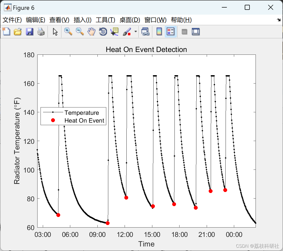
% It looks like I can detect those peaks by looking for large jumps in the
% temperature. After some trial and error, I settled on three criteria to
% identify when the heat comes on:
%
% # Change in temperature greater than four times the previous change in temperature.
% # Change in temperature of more than 1 degree F.
% # Keep the first in a sequence of matching points (remove doubles)
fourtimes = [tempChange(2:end)>abs(4*tempChange(1:end-1)); false];
greaterthanone = [tempChange(2:end)>1; false];
heaton = fourtimes & greaterthanone;
doubles = [false; heaton(2:end) & heaton(1:end-1)];
heaton(doubles) = false;
%%
% Let's see how well I detected those peaks by superimposing red dots over
% the times I detected.
figure
plot(ts,radiatorTemp,'k.-')
hold on
plot(ts(heaton),radiatorTemp(heaton),'r.','MarkerSize',20)
xlim(oneday);
datetick('keeplimits')
xlabel('Time')
ylabel('Radiator Temperature (\circF)')
title('Heat On Event Detection')
legend({'Temperature', 'Heat On Event'},'Location','Best')
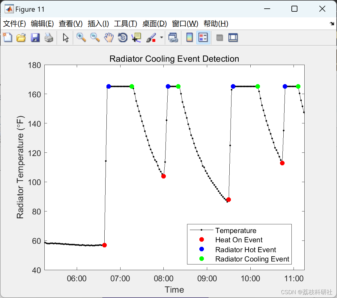
%%
% _Figure 7: Radiator temperature with heating events marked with red dots._
%
% Looks pretty good, which means now I have a list of all the times that
% the heat came on in my apartment.
heatontimes = ts(heaton);
%% How long does it take for my heat to turn on?
% I currently have a programmable 5/2 thermostat, which means I can set
% one program for weekdays (Monday through Friday) and one program for both
% Saturday and Sunday. I know my thermostat is set to go down to 62 at
% night, and back up to 68 at 6:15am Monday through Friday and 10:00am on
% Saturday and Sunday. I used that knowledge to determine how long after my
% thermostat activates that my radiators warm up.
%
% I started by creating a vector of all the days in the test period. I
% removed Monday because I manually turned on the thermostat early that day.
mornings = floor(min(ts)):floor(max(ts));
mornings(2) = []; % Remove Monday
%%
% Then I added either 6:15am or 10:00am to each day depending on whether it
% was a weekday or a weekend.
isweekend = weekday(mornings) == 1 | weekday(mornings) == 7;
mornings(isweekend) = mornings(isweekend)+10/24; % 10:00 AM
mornings(~isweekend) = mornings(~isweekend)+6.25/24; % 6:15 AM
%%
% Next I looked for the first time the heat came on after the programmed
% time each morning.
heatontimes_mat = repmat(heatontimes,1,length(mornings));
mornings_mat = repmat(mornings,length(heatontimes),1);
timelag = heatontimes_mat - mornings_mat;
timelag(timelag<=0) = NaN;
plot(ts,radiatorTemp,'k.-')
hold on
plot(heatontimes,heatontemp,'r.','MarkerSize',20)
plot(heatontimes(heatind),heatontemp(heatind),'bo','MarkerSize',10)
plot([mornings;mornings],repmat(ylim',1,length(mornings)),'b-');
xlim(onemorning);
datetick('keeplimits')
xlabel('Time')
ylabel('Radiator Temperature (\circF)')
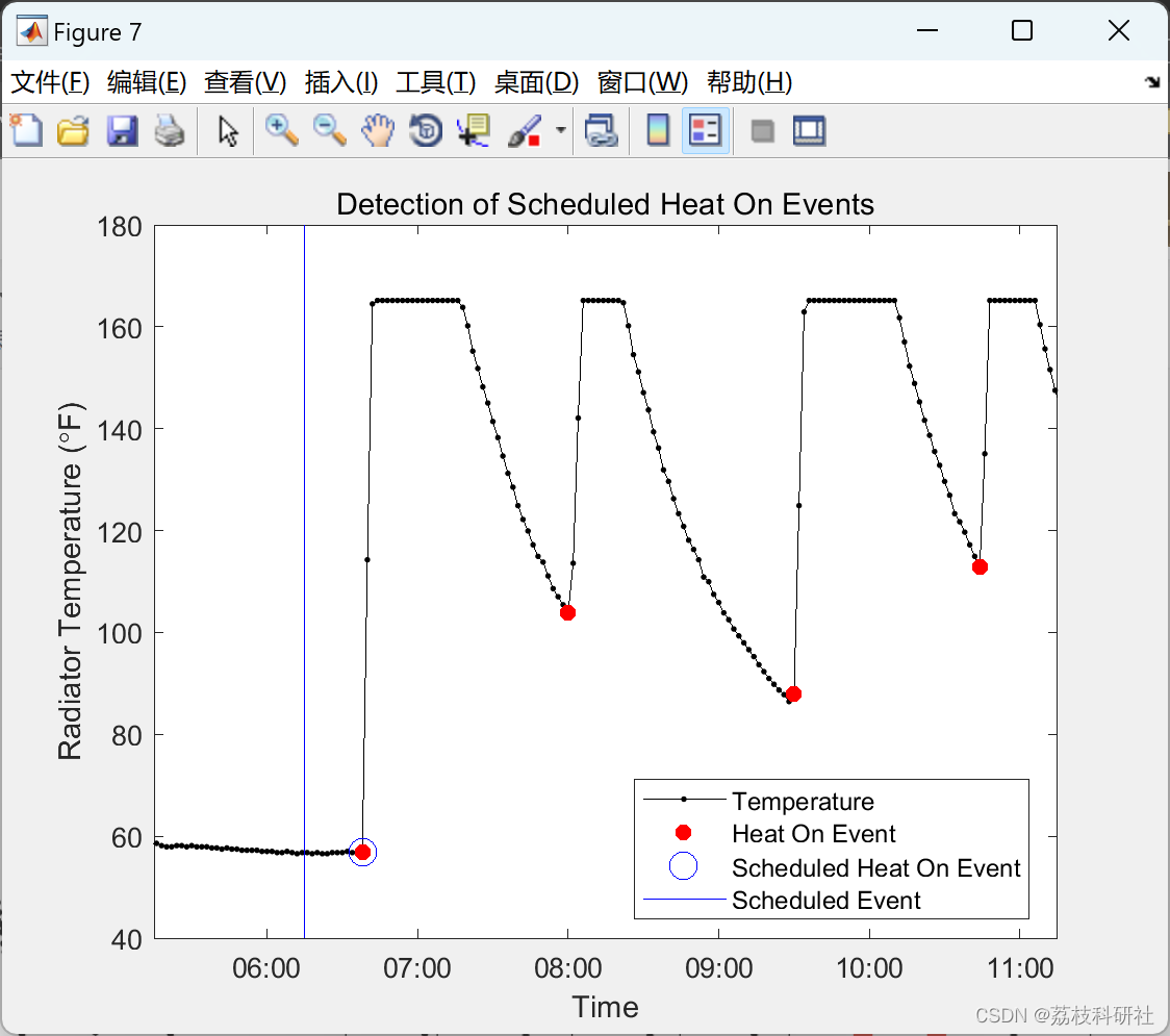
title('Detection of Scheduled Heat On Events')
legend({'Temperature', 'Heat On Event', 'Scheduled Heat On Event',...
'Scheduled Event'},'Location','Best')
%%
% _Figure 8: Six hours of radiator data, with a blue line indicating when
% the thermostat turned on in the morning, and blue circle indicating the
% corresponding heat on event of the radiator._
%
% Let's look at a histogram of those delays:
figure
hist(delay,min(delay):max(delay))
xlabel('Minutes')
ylabel('Frequency')
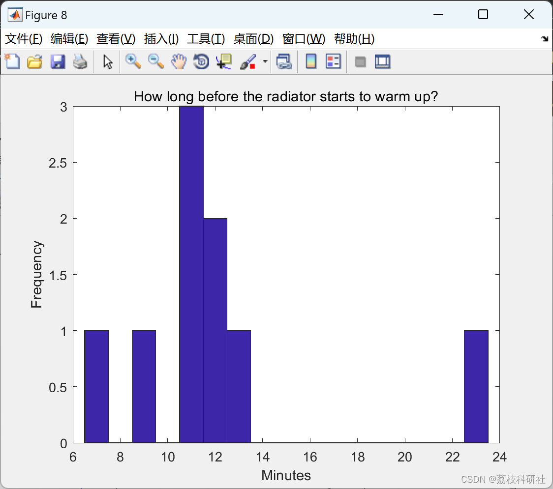
title('How long before the radiator starts to warm up?')
%%
% _Figure 9: Histogram showing delay between thermostat activation and the
% radiators starting to warm up._
%
% It looks like the delay between the thermostat coming on in the morning
% and the radiators starting to warming up can range from 7 minutes to as
% high as 24 minutes, but on average this delay is around 12-13 minutes.
heatondelay = 12;
%% How long does it take for the radiators to warm up?
% Once the radiators start to warm up, it takes a few minutes for them to
% reach full temperature. Let's look at how long this takes. I'll look for
% times when the radiator temperature first maxes out the temperature
% sensor after having been below the maximum for at least 10 minutes (5
% samples).
maxtemp = max(radiatorTemp);
radiatorhot = radiatorTemp(6:end)==maxtemp & ...
radiatorTemp(1:end-5)<maxtemp &...
radiatorTemp(2:end-4)<maxtemp &...
radiatorTemp(3:end-3)<maxtemp &...
radiatorTemp(4:end-2)<maxtemp &...
radiatorTemp(5:end-1)<maxtemp;
radiatorhot = [false(5,1); radiatorhot];
radiatorhottimes = ts(radiatorhot);
%
% Now I'll match the |radiatorhottimes| to the |heatontimes| using the same
% technique I used above.
radiatorhottimes_mat = repmat(radiatorhottimes',length(heatontimes),1);
heatontimes_mat = repmat(heatontimes,1,length(radiatorhottimes));
timelag = radiatorhottimes_mat - heatontimes_mat;
timelag(timelag<=0) = NaN;
[delay, foundmatch] = min(timelag);
delay = round(delay*24*60);
%%
% Let's look at a histogram of those delays:
figure
hist(delay,min(delay):2:max(delay))
xlabel('Minutes');
ylabel('Frequency')
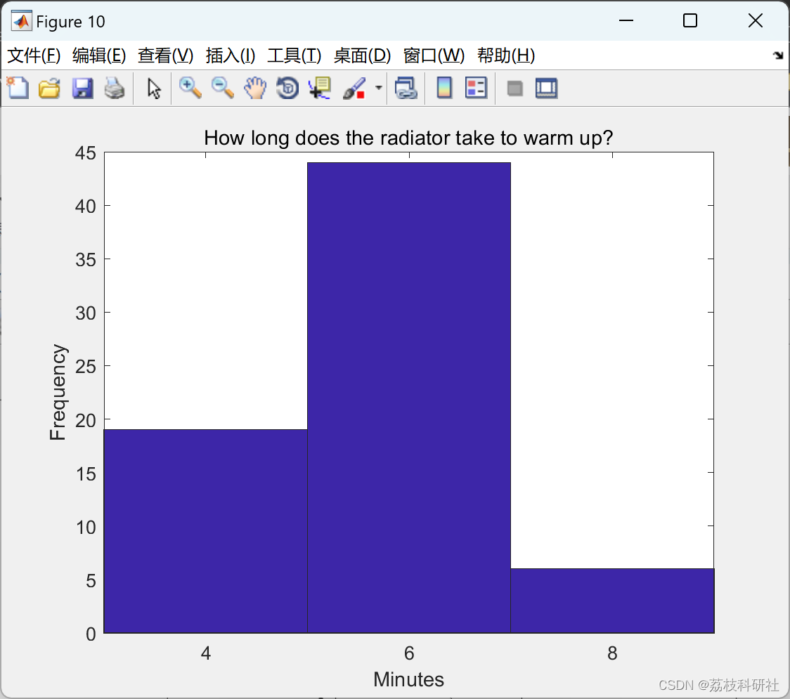
title('How long does the radiator take to warm up?')
%%
% _Figure 11: Histogram showing time required for the radiators to warm up._
%
% It looks like the radiators take between 4 and 8 minutes from when they
% start to warm up until they are at full temperature.
radiatorheatdelay = 6;
%%
% Later on in my analysis, I will only want to use times that the heat came
%
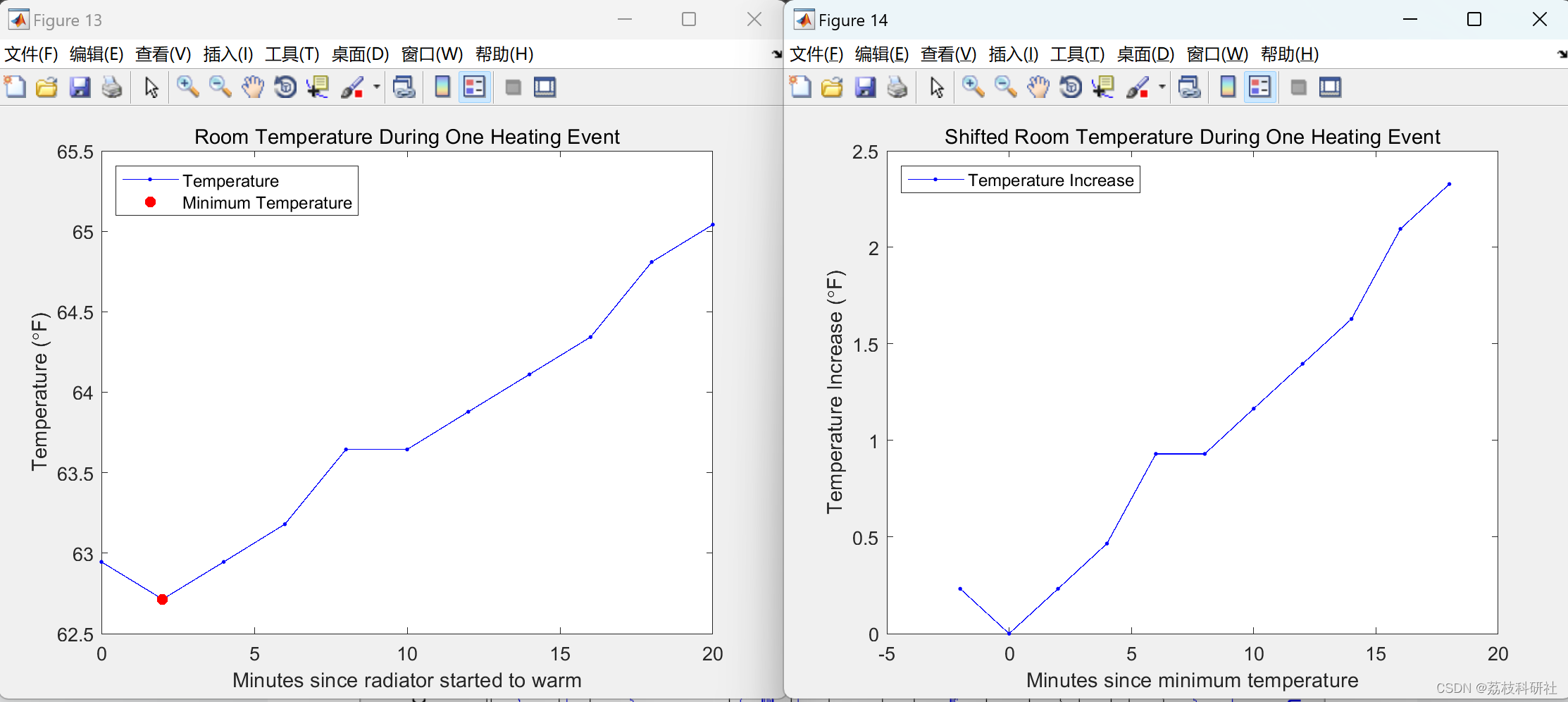
% Although it isn't perfect, it looks close to a linear relationship. Since
% I am interested in the time it takes to reach the desired temperature
% (what could be considered the "specific heat capacity" of the room), let
% me replot the data with time on the y-axis and temperature on the x-axis
% (swapping the axes from the previous figure). I'll also plot the data as
% individual points instead of lines, because that is how the data is going
% to be fed into |polyfit| later.
% Remove temperatures occuring before the minimum temperature.
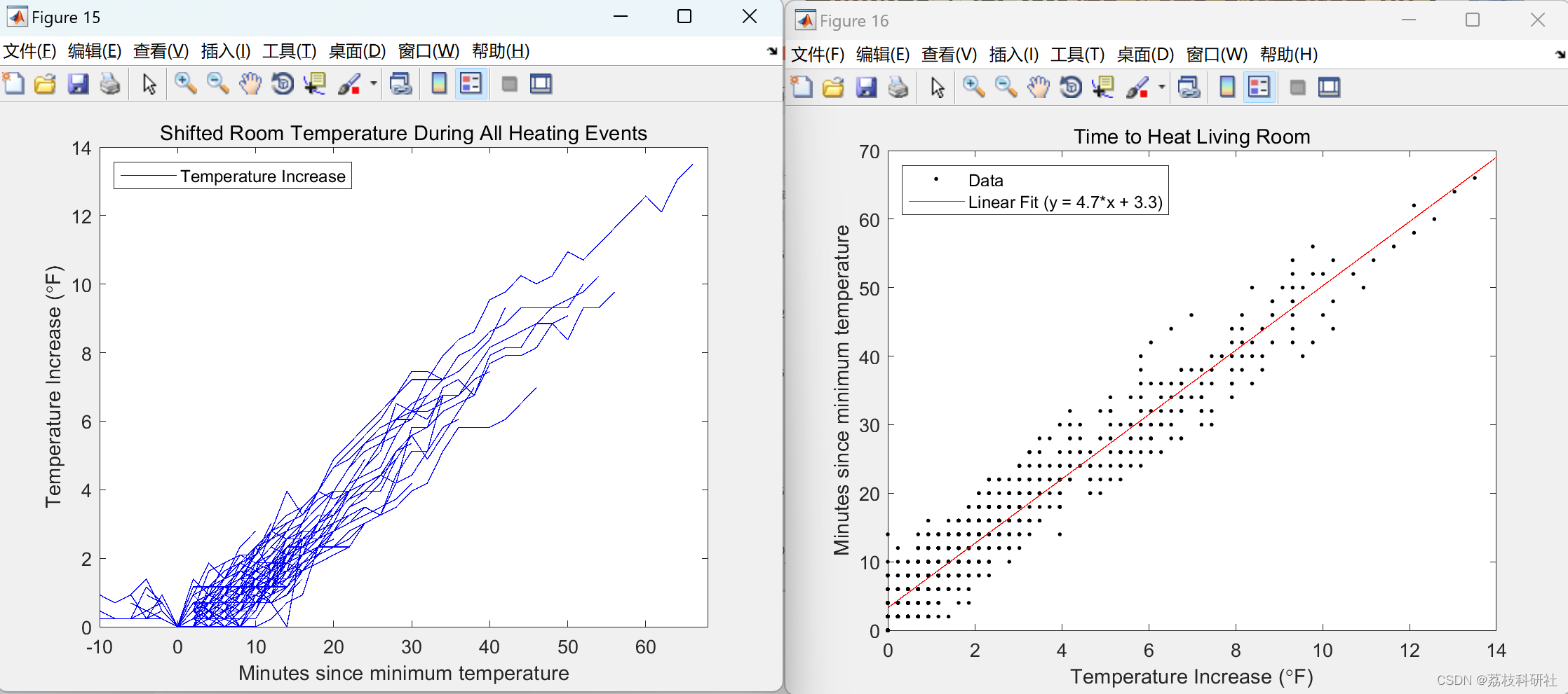
segmentTempsShifted(segmentTimesShifted<0) = NaN;
figure
h1 = plot(segmentTempsShifted',segmentTimesShifted','k.');
xlabel('Temperature Increase (\circF)')
ylabel('Minutes since minimum temperature')
title('Time to Heat Living Room')
snapnow
%%
% _Figure 17: The time it takes to heat the living room (axes flipped from
% Figure 16)._
%
% Now let me fit a line to the data so I can get an equation for the time
% it takes to heat the living room.
%%
% First I collect all the time and temperature data into a single column
% vector and remove |NaN| values.
allTimes = segmentTimesShifted(:);
allTemps = segmentTempsShifted(:);
allTimes(isnan(allTemps)) = [];
allTemps(isnan(allTemps)) = [];
%%
% Then I can fit a line to the data.
linfit = polyfit(allTemps,allTimes,1);
%%
% Let's see how well we fit the data.
hold on
h2 = plot(xlim,polyval(linfit,xlim),'r-');
linfitstr = sprintf('Linear Fit (y = %.1f*x + %.1f)',linfit(1),linfit(2));
legend([ h1(1), h2(1) ],{'Data',linfitstr},'Location','NorthWest')
%%
% _Figure 18: The time it takes to heat the living room along with a linear fit to the data._
%
% Not a bad fit. Looking closer at the coefficients from the linear fit, it
% looks like it takes about 3 minutes after the radiators start to heat up
% for the room to start to warm up. After that, it takes about 5 minutes
% for each degree of temperature increase.
%% What room takes the longest to warm up?
% I can apply the techniques above to each room to find out how long each
% room takes to warm up. I took the code above and put it into a separate
% function called <../temperatureAnalysis.m |temperatureAnalysis|>, and
% applied that to each inside temperature sensor.
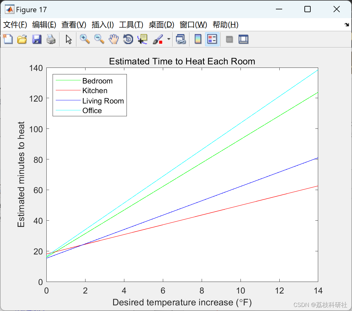
inside = [1 5 9 12];
figure
xl = [0 14];
for s = 1:size(inside,2)
linfits(s,1:2) = temperatureAnalysis(tempF(:,inside(s)), heaton, heatoff);
y = polyval(linfits(s,1:2),xl) + heatondelay;
plot(xl, y, lineSpecs{inside(s),1}, 'Color',lineSpecs{inside(s),2},...
'DisplayName',location{inside(s)})
hold on
end
legend('Location','NorthWest')
xlabel('Desired temperature increase (\circF)')
ylabel('Estimated minutes to heat')
title('Estimated Time to Heat Each Room')
%%
% _Figure 19: The estimated time it takes to heat each room in my apartment._
🎉3 参考文献
部分理论来源于网络,如有侵权请联系删除。
[1]王晓银.基于XBee的瓦斯无线传感器网络节点的设计[J].自动化技术与应用,2018,37(08):46-49.
[2]王晓银.基于XBee的瓦斯无线传感器网络节点的设计[J].自动化技术与应用,2018,37(08):46-49.
🌈4 Matlab代码及数据
相关文章:
【无线传感器】使用 MATLAB和 XBee连续监控温度传感器无线网络研究(Matlab代码实现)
💥💥💞💞欢迎来到本博客❤️❤️💥💥 🏆博主优势:🌞🌞🌞博客内容尽量做到思维缜密,逻辑清晰,为了方便读者。 ⛳️座右铭&a…...
Java基础-多线程JUC-生产者和消费者
1. 生产者与消费者 实现线程轮流交替执行的结果; 实现线程休眠和唤醒均要使用到锁对象; 修改标注位(foodFlag); 代码实现: public class demo11 {public static void main(String[] args) {/*** 需求&#…...
day2 QT按钮与容器
目录 按钮 1、QPushButton 2、QToolButton 3、QRadioButton 4、QCheckBox 示例 容器 编辑 1. QGroupBox(分组框) 2. QScrollArea(滚动区域) 3. QToolBox(工具箱) 4. QTabWidget(选…...
JPA 批量插入较大数据 解决性能慢问题
JPA 批量插入较大数据 解决性能慢问题 使用jpa saveAll接口的话需要了解原理: TransactionalOverridepublic <S extends T> List<S> saveAll(Iterable<S> entities) {Assert.notNull(entities, "Entities must not be null!");List<…...

为啥离不了 linux
Linux与Windows都是十分常见的电脑操作系统,相信你对它们二者都有所了解!在你的使用过程中,是否有什么事让你觉得在Linux上顺理成章,换到Windows上就令你费解?亦或者关于这二者你有任何想要分享的,都可以在…...

基于分形的置乱算法和基于混沌系统的置乱算法哪种更安全?
在信息安全领域中,置乱算法是一种重要的加密手段,它可以将明文进行混淆和打乱,从而实现保密性和安全性。常见的置乱算法包括基于分形的置乱算法和基于混沌系统的置乱算法。下面将从理论和实践两方面,对这两种置乱算法进行比较和分…...

pve使用cloud-image创建ubuntu模板
首先连接pve主机的终端 下载ubuntu22.04的cloud-image镜像 wget -P /opt https://mirrors.cloud.tencent.com/ubuntu-cloud-images/jammy/current/jammy-server-cloudimg-amd64.img创建虚拟机,id设为9000,使用VirtIO SCSI控制器 qm create 9000 -core…...
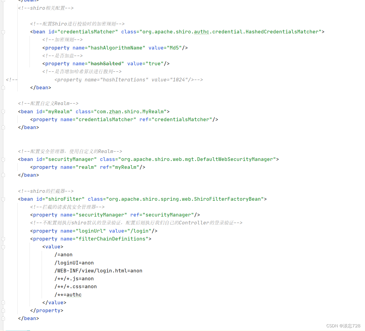
shiro入门
1、概述 Apache Shiro 是一个功能强大且易于使用的 Java 安全(权限)框架。借助 Shiro 您可以快速轻松地保护任何应用程序一一从最小的移动应用程序到最大的 Web 和企业应用程序。 作用:Shiro可以帮我们完成 :认证、授权、加密、会话管理、与 Web 集成、…...
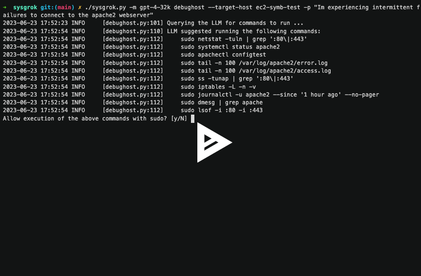
开源 sysgrok — 用于分析、理解和优化系统的人工智能助手
作者:Sean Heelan 在这篇文章中,我将介绍 sysgrok,这是一个研究原型,我们正在研究大型语言模型 (LLM)(例如 OpenAI 的 GPT 模型)如何应用于性能优化、根本原因分析和系统工程领域的问题。 你可以在 GitHub …...

Gitlab保护分支与合并请求
目录 引言 1、成员角色指定 1、保护分支设置 2、合并请求 引言 熟悉了Git工作流之后,有几个重要的分支,如Master(改名为Main)、Develop、Release分支等,是禁止开发成员随意合并和提交的,在此分支上的提交和推送权限仅限项目负责…...

ad18学习笔记九:输出文件
一般来说提供给板卡厂的文件里要包括以下这些文件 1、装配图 2、bom文件 3、gerber文件 4、转孔文件 5、坐标文件 6、ipc网表 AD_PCB:Gerber等各类文件的输出 - 哔哩哔哩 原点|钻孔_硬件设计AD 生成 Gerber 文件 1、装配图 如何输出装配图? 【…...

PostgreSQL 内存配置 与 MemoryContext 的生命周期
PostgreSQL 内存配置与MemoryContext的生命周期 PG/GP 内存配置 数据库可用的内存 gp_vmem 整个 GP 数据库可用的内存 gp_vmem: >>> RAM 128 * GB >>> gp_vmem ((SWAP RAM) - (7.5*GB 0.05 * RAM)) / 1.7 >>> print(gp_vmem / G…...
)
vue3 组件间通信的方式(setup语法糖写法)
vue3 组件间通信的方式(setup语法糖写法) 1. Props方式 该方式用于父传子,父组件以数据绑定的形式声明要传递的数据,子组件通过defineProps()方法创建props对象,即可拿到父组件传来的数据。 // 父组件 <template><div><son…...

【Cache】Rsync远程同步
文章目录 一、rsync 概念二、rysnc 服务器部署1. 环境配置2. rysnc 同步源服务器2.1 安装 rsync2.2 建立 rsyncd.conf 配置文件2.3 创建数据文件(账号密码)2.4 启动服务2.5 数据配置 3. rysnc 客户端3.1 设置同步方法一方法二 3.2 免交互设置 4. rysnc 认…...

Gitlab升级报错一:rails_migration[gitlab-rails] (gitlab::database_migrations line 51)
Gitlab-ce从V14.0.12升级到V14.3.6或V14.10.5时报错:如下图: 解决办法: 先停掉gitlab: gitlab-ctl stop 单独启动数据库,如果不单独启动数据库,就会报以上错误 sudo gitlab-ctl start postgresql 解决办法&#x…...
chatGPT流式回复是怎么实现的
chatGPT流式回复是怎么实现的 先说结论: chatGPT的流式回复用的就是HTTP请求方案中的server-send-event流式接口,也就是服务端向客户端推流数据。 那eventStream流式接口怎么实现呢,下面就进入正题! 文章目录 chatGPT流式回复…...
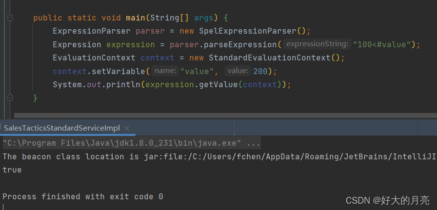
使用SpringEL获得字符串中的表达式运算结果
概述 有时候会遇上奇怪的需求,比如解析字符串中表达式的结果。 这个时候自己写解析肯定是比较麻烦的, 正好SprinngEL支持加()、减(-)、乘(*)、除(/)、求余(%)、幂(^)运算,可以免去造轮子的功夫…...
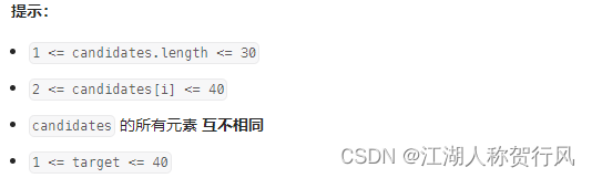
力扣 39. 组合总和
题目来源:https://leetcode.cn/problems/combination-sum/description/ C题解: 递归法。递归前对数组进行有序排序,可方便后续剪枝操作。 递归函数参数:定义两个全局变量,二维数组result存放结果集,数组pa…...
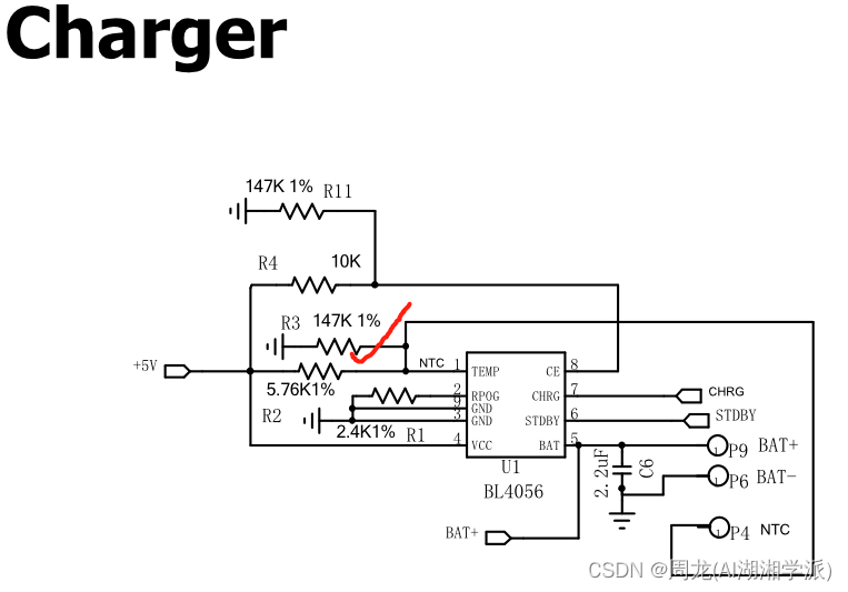
基于BES系列蓝牙耳机NTC充电电池保护电路设计
+hezkz17进数字音频系统研究开发交流答疑 一 在充电电路中NTC作用? 在充电电路中,NTC(Negative Temperature Coefficient)热敏电阻通常被用于温度检测和保护。它具有随温度变化而变化的电阻值。 以下是NTC在充电电路中的几种常见作用: 温度监测:NTC热敏电阻可以用来测量…...

13-C++算法笔记-递归
📚 Introduction 递归是一种常用的算法设计和问题求解方法。它基于问题可以分解为相同类型的子问题,并通过解决子问题来解决原始问题的思想。递归算法在实际编程中具有广泛的应用。 🎯 递归算法解决问题的特点 递归算法具有以下特点&#…...

深度强化学习优化量子比特反馈控制:从DQN原理到实验部署
1. 项目概述与核心价值最近在实验室里折腾一个挺有意思的课题,就是怎么用强化学习去优化量子比特的测量和反馈控制。听起来有点跨界,对吧?量子计算和强化学习,一个在微观世界玩叠加和纠缠,一个在宏观世界搞决策和优化&…...

AI时代知识工作者的创造力转型:从内容生产到批判性整合
1. 项目概述:当AI成为你的“副驾驶”,知识工作者的创造力何去何从?如果你是一位文案、设计师、程序员,或者任何一位以“生产内容”为核心的知识工作者,最近一两年,你大概率已经和ChatGPT、Midjourney、GitH…...

Strada.Brain:基于PAOR循环与多智能体编排的Unity AI编程副驾驶
1. 项目概述:一个为Unity开发者服务的AI编程副驾驶 如果你是一个Unity开发者,或者正在用C#做游戏,每天在编辑器、脚本和构建错误之间反复横跳,那今天聊的这个东西可能会让你眼前一亮。Strada.Brain,这名字听起来有点科…...

CANN/atvoss 项目目录结构
Atvoss 项目目录结构说明 【免费下载链接】atvoss ATVOSS(Ascend C Templates for Vector Operator Subroutines)是一套基于Ascend C开发的Vector算子库,致力于为昇腾硬件上的Vector类融合算子提供极简、高效、高性能、高拓展的编程方式。 …...

CubiFS容器存储备份与恢复:终极完整指南
CubiFS容器存储备份与恢复:终极完整指南 【免费下载链接】cubefs cloud-native distributed storage 项目地址: https://gitcode.com/gh_mirrors/cu/cubefs 在云原生时代,数据安全性和可靠性是企业级存储系统的生命线。CubiFS容器存储备份与恢复机…...

CANN/shmem编译构建指南
编译与构建 【免费下载链接】shmem CANN SHMEM 是面向昇腾平台的多机多卡内存通信库,基于OpenSHMEM 标准协议,实现跨设备的高效内存访问与数据同步。 项目地址: https://gitcode.com/cann/shmem SHMEM编译 下载SHMEM源码 git clone https://git…...

5分钟让小爱音箱变身AI语音助手:MiGPT完整指南
5分钟让小爱音箱变身AI语音助手:MiGPT完整指南 【免费下载链接】mi-gpt 🏠 将小爱音箱接入 ChatGPT 和豆包,改造成你的专属语音助手。 项目地址: https://gitcode.com/GitHub_Trending/mi/mi-gpt 你是否曾经对着小爱音箱提问ÿ…...

ChatGPT与CAQDAS融合:人机协同定性分析工作流实战指南
1. 项目概述:当AI遇到定性研究,一场效率革命“定性分析”这四个字,对于社会学、人类学、心理学、教育学乃至市场研究领域的从业者来说,往往意味着海量的访谈录音、成堆的观察笔记、以及无数个在文本中反复爬梳、编码、寻找模式的深…...

大语言模型推理能力与自指认知的架构解析
1. 大语言模型推理能力的底层架构解析大语言模型的逻辑推理能力建立在Transformer架构的多层自注意力机制之上。这种架构设计使得模型能够通过注意力权重动态构建不同概念之间的关联网络。在推理任务中,特定模式的注意力分布会形成类似人类"思维链"的信息…...

CANN/ops-cv算子跨平台迁移指导
算子跨平台迁移指导 【免费下载链接】ops-cv 本项目是CANN提供的图像处理、目标检测相关的算子库,实现网络在NPU上加速计算。 项目地址: https://gitcode.com/cann/ops-cv 本指南介绍算子在多平台间迁移的适配要点与方案。以算子从Atlas A2系列迁移至Ascend …...