【机器学习】Cost Function for Logistic Regression
Cost Function for Logistic Regression
- 1. 平方差能否用于逻辑回归?
- 2. 逻辑损失函数loss
- 3. 损失函数cost
- 附录
导入所需的库
import numpy as np
%matplotlib widget
import matplotlib.pyplot as plt
from plt_logistic_loss import  plt_logistic_cost, plt_two_logistic_loss_curves, plt_simple_example
from plt_logistic_loss import soup_bowl, plt_logistic_squared_error
from lab_utils_common import  plot_data, sigmoid, dlc
plt.style.use('./deeplearning.mplstyle')
1. 平方差能否用于逻辑回归?
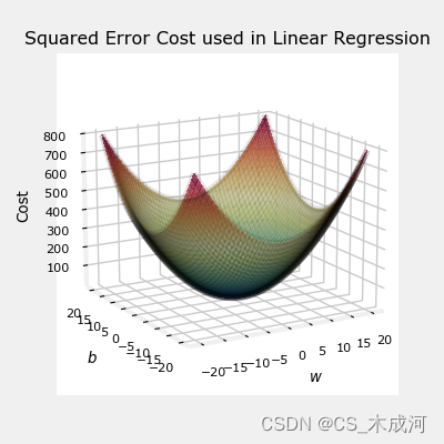
在前面的线性回归中,我们使用的是 squared error cost function,带有一个变量的squared error cost 为:
J ( w , b ) = 1 2 m ∑ i = 0 m − 1 ( f w , b ( x ( i ) ) − y ( i ) ) 2 (1) J(w,b) = \frac{1}{2m} \sum\limits_{i = 0}^{m-1} (f_{w,b}(x^{(i)}) - y^{(i)})^2 \tag{1} J(w,b)=2m1i=0∑m−1(fw,b(x(i))−y(i))2(1)
其中,
f w , b ( x ( i ) ) = w x ( i ) + b (2) f_{w,b}(x^{(i)}) = wx^{(i)} + b \tag{2} fw,b(x(i))=wx(i)+b(2)
squared error cost有一个很好的性质,就是对cost求导会得到最小值。
soup_bowl()
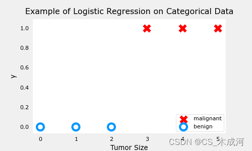
这个cost函数在线性回归中表现得很好,当然,它也适用于逻辑回归。然而, f w b ( x ) f_{wb}(x) fwb(x)现在有一个非线性的部分,即sigmoid函数: f w , b ( x ( i ) ) = s i g m o i d ( w x ( i ) + b ) f_{w,b}(x^{(i)}) = sigmoid(wx^{(i)} + b ) fw,b(x(i))=sigmoid(wx(i)+b)。接下来,我们尝试使用squared error cost在以前博客的样例中,此时包括sigmod。
训练数据:
x_train = np.array([0., 1, 2, 3, 4, 5],dtype=np.longdouble)
y_train = np.array([0,  0, 0, 1, 1, 1],dtype=np.longdouble)
plt_simple_example(x_train, y_train)
现在,用squared error cost 绘制cost的曲面图:
J ( w , b ) = 1 2 m ∑ i = 0 m − 1 ( f w , b ( x ( i ) ) − y ( i ) ) 2 J(w,b) = \frac{1}{2m} \sum\limits_{i = 0}^{m-1} (f_{w,b}(x^{(i)}) - y^{(i)})^2 J(w,b)=2m1i=0∑m−1(fw,b(x(i))−y(i))2
其中,
f w , b ( x ( i ) ) = s i g m o i d ( w x ( i ) + b ) f_{w,b}(x^{(i)}) = sigmoid(wx^{(i)} + b ) fw,b(x(i))=sigmoid(wx(i)+b)
plt.close('all')
plt_logistic_squared_error(x_train,y_train)
plt.show()
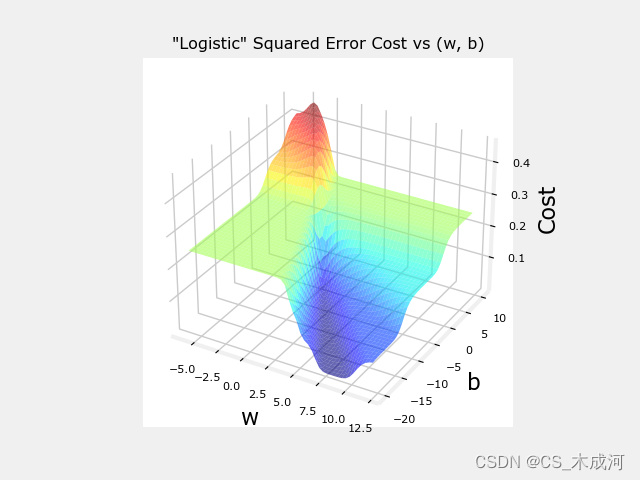
虽然这产生了一个非常有趣的曲面图,但上面的曲面并不像线性回归的“汤碗”那么光滑。逻辑回归需要一个更适合其非线性性质的cost函数。
2. 逻辑损失函数loss
逻辑回归使用更适合分类任务的Loss函数,其中目标是0或1而不是任何数字。
注意:Loss是单个示例与其目标值之差的度量,而Cost是训练集上损失的度量。
定义: l o s s ( f w , b ( x ( i ) ) , y ( i ) ) loss(f_{\mathbf{w},b}(\mathbf{x}^{(i)}), y^{(i)}) loss(fw,b(x(i)),y(i)) 是单个数据点的cost:
l o s s ( f w , b ( x ( i ) ) , y ( i ) ) = { − log ( f w , b ( x ( i ) ) ) if y ( i ) = 1 log ( 1 − f w , b ( x ( i ) ) ) if y ( i ) = 0 \begin{equation} loss(f_{\mathbf{w},b}(\mathbf{x}^{(i)}), y^{(i)}) = \begin{cases} - \log\left(f_{\mathbf{w},b}\left( \mathbf{x}^{(i)} \right) \right) & \text{if $y^{(i)}=1$}\\ \log \left( 1 - f_{\mathbf{w},b}\left( \mathbf{x}^{(i)} \right) \right) & \text{if $y^{(i)}=0$} \end{cases} \end{equation} loss(fw,b(x(i)),y(i))={−log(fw,b(x(i)))log(1−fw,b(x(i)))if y(i)=1if y(i)=0
f w , b ( x ( i ) ) f_{\mathbf{w},b}(\mathbf{x}^{(i)}) fw,b(x(i)) 是模型的预测值, y ( i ) y^{(i)} y(i) 是目标值.
f w , b ( x ( i ) ) = g ( w ⋅ x ( i ) + b ) f_{\mathbf{w},b}(\mathbf{x}^{(i)}) = g(\mathbf{w} \cdot\mathbf{x}^{(i)}+b) fw,b(x(i))=g(w⋅x(i)+b) ,其中 g g g 是 sigmoid 函数.
这个损失函数的定义特点在于使用了两条不同的曲线。一个用于目标为0或( y = 0 y=0 y=0)的情况,另一个用于目标为1 ( y = 1 y=1 y=1)的情况。这些曲线结合起来为损失函数提供了帮助,即当预测与目标匹配时为零,当预测与目标不同时 l o s s loss loss 值迅速增加。
plt_two_logistic_loss_curves()
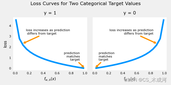
综合起来,曲线类似于平方差损失的二次曲线。注意,x轴是 f w , b f_{\mathbf{w},b} fw,b,是sigmoid的输出。sigmoid 输出严格在0到1之间。
上面的损失函数可以简写为:
l o s s ( f w , b ( x ( i ) ) , y ( i ) ) = ( − y ( i ) log ( f w , b ( x ( i ) ) ) − ( 1 − y ( i ) ) log ( 1 − f w , b ( x ( i ) ) ) loss(f_{\mathbf{w},b}(\mathbf{x}^{(i)}), y^{(i)}) = (-y^{(i)} \log\left(f_{\mathbf{w},b}\left( \mathbf{x}^{(i)} \right) \right) - \left( 1 - y^{(i)}\right) \log \left( 1 - f_{\mathbf{w},b}\left( \mathbf{x}^{(i)} \right) \right) loss(fw,b(x(i)),y(i))=(−y(i)log(fw,b(x(i)))−(1−y(i))log(1−fw,b(x(i)))
可以将方程分成两部分:
当 y ( i ) = 0 y^{(i)} = 0 y(i)=0 时,左边的项被消除:
l o s s ( f w , b ( x ( i ) ) , 0 ) = ( − ( 0 ) log ( f w , b ( x ( i ) ) ) − ( 1 − 0 ) log ( 1 − f w , b ( x ( i ) ) ) = − log ( 1 − f w , b ( x ( i ) ) ) \begin{align} loss(f_{\mathbf{w},b}(\mathbf{x}^{(i)}), 0) &= (-(0) \log\left(f_{\mathbf{w},b}\left( \mathbf{x}^{(i)} \right) \right) - \left( 1 - 0\right) \log \left( 1 - f_{\mathbf{w},b}\left( \mathbf{x}^{(i)} \right) \right) \\ &= -\log \left( 1 - f_{\mathbf{w},b}\left( \mathbf{x}^{(i)} \right) \right) \end{align} loss(fw,b(x(i)),0)=(−(0)log(fw,b(x(i)))−(1−0)log(1−fw,b(x(i)))=−log(1−fw,b(x(i)))
当 y ( i ) = 1 y^{(i)} = 1 y(i)=1 时, 右边的项被消除:
l o s s ( f w , b ( x ( i ) ) , 1 ) = ( − ( 1 ) log ( f w , b ( x ( i ) ) ) − ( 1 − 1 ) log ( 1 − f w , b ( x ( i ) ) ) = − log ( f w , b ( x ( i ) ) ) \begin{align} loss(f_{\mathbf{w},b}(\mathbf{x}^{(i)}), 1) &= (-(1) \log\left(f_{\mathbf{w},b}\left( \mathbf{x}^{(i)} \right) \right) - \left( 1 - 1\right) \log \left( 1 - f_{\mathbf{w},b}\left( \mathbf{x}^{(i)} \right) \right)\\ &= -\log\left(f_{\mathbf{w},b}\left( \mathbf{x}^{(i)} \right) \right) \end{align} loss(fw,b(x(i)),1)=(−(1)log(fw,b(x(i)))−(1−1)log(1−fw,b(x(i)))=−log(fw,b(x(i)))
所以,我们可以通过这个新的逻辑损失函数得到一个包含所有样例的损失函数。
上面示例的损失与参数曲线为:
plt.close('all')
cst = plt_logistic_cost(x_train,y_train)
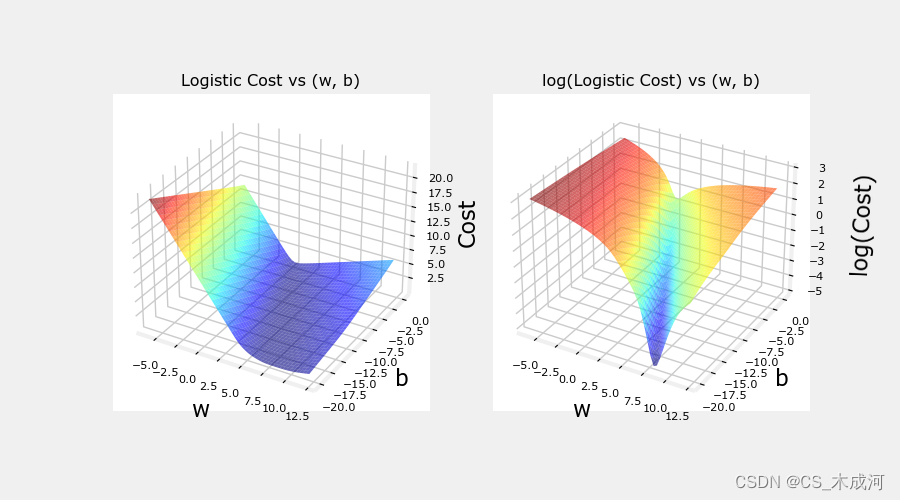
这条曲线非常适合梯度下降。它没有局部极小值或不连续点。需要注意的是,它不像平方差损失那样呈现“碗”状。绘制cost和log cost来说明,当cost较小时,曲线有一个斜率并继续下降。
3. 损失函数cost
导入数据集
X_train = np.array([[0.5, 1.5], [1,1], [1.5, 0.5], [3, 0.5], [2, 2], [1, 2.5]])  #(m,n)
y_train = np.array([0, 0, 0, 1, 1, 1])                                           #(m,)
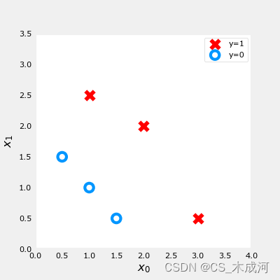
训练数据绘图可视化:
fig,ax = plt.subplots(1,1,figsize=(4,4))
plot_data(X_train, y_train, ax)# Set both axes to be from 0-4
ax.axis([0, 4, 0, 3.5])
ax.set_ylabel('$x_1$', fontsize=12)
ax.set_xlabel('$x_0$', fontsize=12)
plt.show()
前面介绍了一个样例的逻辑 loss 函数,这里我们根据 loss 计算包括所有样例的cost 。
对于逻辑回归,cost 函数表示为:
J ( w , b ) = 1 m ∑ i = 0 m − 1 [ l o s s ( f w , b ( x ( i ) ) , y ( i ) ) ] (1) J(\mathbf{w},b) = \frac{1}{m} \sum_{i=0}^{m-1} \left[ loss(f_{\mathbf{w},b}(\mathbf{x}^{(i)}), y^{(i)}) \right] \tag{1} J(w,b)=m1i=0∑m−1[loss(fw,b(x(i)),y(i))](1)
其中,
- l o s s ( f w , b ( x ( i ) ) , y ( i ) ) loss(f_{\mathbf{w},b}(\mathbf{x}^{(i)}), y^{(i)}) loss(fw,b(x(i)),y(i)) 是一个单独数据点的cost,即:
l o s s ( f w , b ( x ( i ) ) , y ( i ) ) = − y ( i ) log ( f w , b ( x ( i ) ) ) − ( 1 − y ( i ) ) log ( 1 − f w , b ( x ( i ) ) ) (2) loss(f_{\mathbf{w},b}(\mathbf{x}^{(i)}), y^{(i)}) = -y^{(i)} \log\left(f_{\mathbf{w},b}\left( \mathbf{x}^{(i)} \right) \right) - \left( 1 - y^{(i)}\right) \log \left( 1 - f_{\mathbf{w},b}\left( \mathbf{x}^{(i)} \right) \right) \tag{2} loss(fw,b(x(i)),y(i))=−y(i)log(fw,b(x(i)))−(1−y(i))log(1−fw,b(x(i)))(2)
其中,m是数据集中训练样例的数量。
f w , b ( x ( i ) ) = g ( z ( i ) ) z ( i ) = w ⋅ x ( i ) + b g ( z ( i ) ) = 1 1 + e − z ( i ) \begin{align} f_{\mathbf{w},b}(\mathbf{x^{(i)}}) &= g(z^{(i)})\tag{3} \\ z^{(i)} &= \mathbf{w} \cdot \mathbf{x}^{(i)}+ b\tag{4} \\ g(z^{(i)}) &= \frac{1}{1+e^{-z^{(i)}}}\tag{5} \end{align} fw,b(x(i))z(i)g(z(i))=g(z(i))=w⋅x(i)+b=1+e−z(i)1(3)(4)(5)
其代码描述为:
compute_cost_logistic算法在所有的样例上循环,计算每个样例的损失并相加。
变量 X 和 y 不是标量,而是shape分别为( m , n m, n m,n) 和 ( m m m) 的矩阵。其中 n n n 是特征的数量, m m m 是训练样例的数量.
def compute_cost_logistic(X, y, w, b):"""Computes costArgs:X (ndarray (m,n)): Data, m examples with n featuresy (ndarray (m,)) : target valuesw (ndarray (n,)) : model parameters b (scalar) : model parameterReturns:cost (scalar): cost"""m = X.shape[0]cost = 0.0for i in range(m):z_i = np.dot(X[i],w) + bf_wb_i = sigmoid(z_i)cost += -y[i]*np.log(f_wb_i) - (1-y[i])*np.log(1-f_wb_i)cost = cost / mreturn cost
测试一下:
w_tmp = np.array([1,1])
b_tmp = -3
print(compute_cost_logistic(X_train, y_train, w_tmp, b_tmp))
输出为:0.3668667864055175
附录
lab_utils_common.py 源码:
"""
lab_utils_commoncontains common routines and variable definitionsused by all the labs in this week.by contrast, specific, large plotting routines will be in separate filesand are generally imported into the week where they are used.those files will import this file
"""
import copy
import math
import numpy as np
import matplotlib.pyplot as plt
from matplotlib.patches import FancyArrowPatch
from ipywidgets import Outputnp.set_printoptions(precision=2)dlc = dict(dlblue = '#0096ff', dlorange = '#FF9300', dldarkred='#C00000', dlmagenta='#FF40FF', dlpurple='#7030A0')
dlblue = '#0096ff'; dlorange = '#FF9300'; dldarkred='#C00000'; dlmagenta='#FF40FF'; dlpurple='#7030A0'
dlcolors = [dlblue, dlorange, dldarkred, dlmagenta, dlpurple]
plt.style.use('./deeplearning.mplstyle')def sigmoid(z):"""Compute the sigmoid of zParameters----------z : array_likeA scalar or numpy array of any size.Returns-------g : array_likesigmoid(z)"""z = np.clip( z, -500, 500 )           # protect against overflowg = 1.0/(1.0+np.exp(-z))return g##########################################################
# Regression Routines
##########################################################def predict_logistic(X, w, b):""" performs prediction """return sigmoid(X @ w + b)def predict_linear(X, w, b):""" performs prediction """return X @ w + bdef compute_cost_logistic(X, y, w, b, lambda_=0, safe=False):"""Computes cost using logistic loss, non-matrix versionArgs:X (ndarray): Shape (m,n)  matrix of examples with n featuresy (ndarray): Shape (m,)   target valuesw (ndarray): Shape (n,)   parameters for predictionb (scalar):               parameter  for predictionlambda_ : (scalar, float) Controls amount of regularization, 0 = no regularizationsafe : (boolean)          True-selects under/overflow safe algorithmReturns:cost (scalar): cost"""m,n = X.shapecost = 0.0for i in range(m):z_i    = np.dot(X[i],w) + b                                             #(n,)(n,) or (n,) ()if safe:  #avoids overflowscost += -(y[i] * z_i ) + log_1pexp(z_i)else:f_wb_i = sigmoid(z_i)                                                   #(n,)cost  += -y[i] * np.log(f_wb_i) - (1 - y[i]) * np.log(1 - f_wb_i)       # scalarcost = cost/mreg_cost = 0if lambda_ != 0:for j in range(n):reg_cost += (w[j]**2)                                               # scalarreg_cost = (lambda_/(2*m))*reg_costreturn cost + reg_costdef log_1pexp(x, maximum=20):''' approximate log(1+exp^x)https://stats.stackexchange.com/questions/475589/numerical-computation-of-cross-entropy-in-practiceArgs:x   : (ndarray Shape (n,1) or (n,)  inputout : (ndarray Shape matches x      output ~= np.log(1+exp(x))'''out  = np.zeros_like(x,dtype=float)i    = x <= maximumni   = np.logical_not(i)out[i]  = np.log(1 + np.exp(x[i]))out[ni] = x[ni]return outdef compute_cost_matrix(X, y, w, b, logistic=False, lambda_=0, safe=True):"""Computes the cost using  using matricesArgs:X : (ndarray, Shape (m,n))          matrix of examplesy : (ndarray  Shape (m,) or (m,1))  target value of each examplew : (ndarray  Shape (n,) or (n,1))  Values of parameter(s) of the modelb : (scalar )                       Values of parameter of the modelverbose : (Boolean) If true, print out intermediate value f_wbReturns:total_cost: (scalar)                cost"""m = X.shape[0]y = y.reshape(-1,1)             # ensure 2Dw = w.reshape(-1,1)             # ensure 2Dif logistic:if safe:  #safe from overflowz = X @ w + b                                                           #(m,n)(n,1)=(m,1)cost = -(y * z) + log_1pexp(z)cost = np.sum(cost)/m                                                   # (scalar)else:f    = sigmoid(X @ w + b)                                               # (m,n)(n,1) = (m,1)cost = (1/m)*(np.dot(-y.T, np.log(f)) - np.dot((1-y).T, np.log(1-f)))   # (1,m)(m,1) = (1,1)cost = cost[0,0]                                                        # scalarelse:f    = X @ w + b                                                        # (m,n)(n,1) = (m,1)cost = (1/(2*m)) * np.sum((f - y)**2)                                   # scalarreg_cost = (lambda_/(2*m)) * np.sum(w**2)                                   # scalartotal_cost = cost + reg_cost                                                # scalarreturn total_cost                                                           # scalardef compute_gradient_matrix(X, y, w, b, logistic=False, lambda_=0):"""Computes the gradient using matricesArgs:X : (ndarray, Shape (m,n))          matrix of examplesy : (ndarray  Shape (m,) or (m,1))  target value of each examplew : (ndarray  Shape (n,) or (n,1))  Values of parameters of the modelb : (scalar )                       Values of parameter of the modellogistic: (boolean)                 linear if false, logistic if truelambda_:  (float)                   applies regularization if non-zeroReturnsdj_dw: (array_like Shape (n,1))     The gradient of the cost w.r.t. the parameters wdj_db: (scalar)                     The gradient of the cost w.r.t. the parameter b"""m = X.shape[0]y = y.reshape(-1,1)             # ensure 2Dw = w.reshape(-1,1)             # ensure 2Df_wb  = sigmoid( X @ w + b ) if logistic else  X @ w + b      # (m,n)(n,1) = (m,1)err   = f_wb - y                                              # (m,1)dj_dw = (1/m) * (X.T @ err)                                   # (n,m)(m,1) = (n,1)dj_db = (1/m) * np.sum(err)                                   # scalardj_dw += (lambda_/m) * w        # regularize                  # (n,1)return dj_db, dj_dw                                           # scalar, (n,1)def gradient_descent(X, y, w_in, b_in, alpha, num_iters, logistic=False, lambda_=0, verbose=True):"""Performs batch gradient descent to learn theta. Updates theta by takingnum_iters gradient steps with learning rate alphaArgs:X (ndarray):    Shape (m,n)         matrix of examplesy (ndarray):    Shape (m,) or (m,1) target value of each examplew_in (ndarray): Shape (n,) or (n,1) Initial values of parameters of the modelb_in (scalar):                      Initial value of parameter of the modellogistic: (boolean)                 linear if false, logistic if truelambda_:  (float)                   applies regularization if non-zeroalpha (float):                      Learning ratenum_iters (int):                    number of iterations to run gradient descentReturns:w (ndarray): Shape (n,) or (n,1)    Updated values of parameters; matches incoming shapeb (scalar):                         Updated value of parameter"""# An array to store cost J and w's at each iteration primarily for graphing laterJ_history = []w = copy.deepcopy(w_in)  #avoid modifying global w within functionb = b_inw = w.reshape(-1,1)      #prep for matrix operationsy = y.reshape(-1,1)for i in range(num_iters):# Calculate the gradient and update the parametersdj_db,dj_dw = compute_gradient_matrix(X, y, w, b, logistic, lambda_)# Update Parameters using w, b, alpha and gradientw = w - alpha * dj_dwb = b - alpha * dj_db# Save cost J at each iterationif i<100000:      # prevent resource exhaustionJ_history.append( compute_cost_matrix(X, y, w, b, logistic, lambda_) )# Print cost every at intervals 10 times or as many iterations if < 10if i% math.ceil(num_iters / 10) == 0:if verbose: print(f"Iteration {i:4d}: Cost {J_history[-1]}   ")return w.reshape(w_in.shape), b, J_history  #return final w,b and J history for graphingdef zscore_normalize_features(X):"""computes  X, zcore normalized by columnArgs:X (ndarray): Shape (m,n) input data, m examples, n featuresReturns:X_norm (ndarray): Shape (m,n)  input normalized by columnmu (ndarray):     Shape (n,)   mean of each featuresigma (ndarray):  Shape (n,)   standard deviation of each feature"""# find the mean of each column/featuremu     = np.mean(X, axis=0)                 # mu will have shape (n,)# find the standard deviation of each column/featuresigma  = np.std(X, axis=0)                  # sigma will have shape (n,)# element-wise, subtract mu for that column from each example, divide by std for that columnX_norm = (X - mu) / sigmareturn X_norm, mu, sigma#check our work
#from sklearn.preprocessing import scale
#scale(X_orig, axis=0, with_mean=True, with_std=True, copy=True)######################################################
# Common Plotting Routines
######################################################def plot_data(X, y, ax, pos_label="y=1", neg_label="y=0", s=80, loc='best' ):""" plots logistic data with two axis """# Find Indices of Positive and Negative Examplespos = y == 1neg = y == 0pos = pos.reshape(-1,)  #work with 1D or 1D y vectorsneg = neg.reshape(-1,)# Plot examplesax.scatter(X[pos, 0], X[pos, 1], marker='x', s=s, c = 'red', label=pos_label)ax.scatter(X[neg, 0], X[neg, 1], marker='o', s=s, label=neg_label, facecolors='none', edgecolors=dlblue, lw=3)ax.legend(loc=loc)ax.figure.canvas.toolbar_visible = Falseax.figure.canvas.header_visible = Falseax.figure.canvas.footer_visible = Falsedef plt_tumor_data(x, y, ax):""" plots tumor data on one axis """pos = y == 1neg = y == 0ax.scatter(x[pos], y[pos], marker='x', s=80, c = 'red', label="malignant")ax.scatter(x[neg], y[neg], marker='o', s=100, label="benign", facecolors='none', edgecolors=dlblue,lw=3)ax.set_ylim(-0.175,1.1)ax.set_ylabel('y')ax.set_xlabel('Tumor Size')ax.set_title("Logistic Regression on Categorical Data")ax.figure.canvas.toolbar_visible = Falseax.figure.canvas.header_visible = Falseax.figure.canvas.footer_visible = False# Draws a threshold at 0.5
def draw_vthresh(ax,x):""" draws a threshold """ylim = ax.get_ylim()xlim = ax.get_xlim()ax.fill_between([xlim[0], x], [ylim[1], ylim[1]], alpha=0.2, color=dlblue)ax.fill_between([x, xlim[1]], [ylim[1], ylim[1]], alpha=0.2, color=dldarkred)ax.annotate("z >= 0", xy= [x,0.5], xycoords='data',xytext=[30,5],textcoords='offset points')d = FancyArrowPatch(posA=(x, 0.5), posB=(x+3, 0.5), color=dldarkred,arrowstyle='simple, head_width=5, head_length=10, tail_width=0.0',)ax.add_artist(d)ax.annotate("z < 0", xy= [x,0.5], xycoords='data',xytext=[-50,5],textcoords='offset points', ha='left')f = FancyArrowPatch(posA=(x, 0.5), posB=(x-3, 0.5), color=dlblue,arrowstyle='simple, head_width=5, head_length=10, tail_width=0.0',)ax.add_artist(f)
plt_logistic_loss.py 源码:
"""----------------------------------------------------------------logistic_loss plotting routines and support
"""from matplotlib import cm
from lab_utils_common import sigmoid, dlblue, dlorange, np, plt, compute_cost_matrixdef compute_cost_logistic_sq_err(X, y, w, b):"""compute sq error cost on logicist data (for negative example only, not used in practice)Args:X (ndarray): Shape (m,n) matrix of examples with multiple featuresw (ndarray): Shape (n)   parameters for predictionb (scalar):              parameter  for predictionReturns:cost (scalar): cost"""m = X.shape[0]cost = 0.0for i in range(m):z_i = np.dot(X[i],w) + bf_wb_i = sigmoid(z_i)                 #add sigmoid to normal sq error cost for linear regressioncost = cost + (f_wb_i - y[i])**2cost = cost / (2 * m)return np.squeeze(cost)def plt_logistic_squared_error(X,y):""" plots logistic squared error for demonstration """wx, by = np.meshgrid(np.linspace(-6,12,50),np.linspace(10, -20, 40))points = np.c_[wx.ravel(), by.ravel()]cost = np.zeros(points.shape[0])for i in range(points.shape[0]):w,b = points[i]cost[i] = compute_cost_logistic_sq_err(X.reshape(-1,1), y, w, b)cost = cost.reshape(wx.shape)fig = plt.figure()fig.canvas.toolbar_visible = Falsefig.canvas.header_visible = Falsefig.canvas.footer_visible = Falseax = fig.add_subplot(1, 1, 1, projection='3d')ax.plot_surface(wx, by, cost, alpha=0.6,cmap=cm.jet,)ax.set_xlabel('w', fontsize=16)ax.set_ylabel('b', fontsize=16)ax.set_zlabel("Cost", rotation=90, fontsize=16)ax.set_title('"Logistic" Squared Error Cost vs (w, b)')ax.xaxis.set_pane_color((1.0, 1.0, 1.0, 0.0))ax.yaxis.set_pane_color((1.0, 1.0, 1.0, 0.0))ax.zaxis.set_pane_color((1.0, 1.0, 1.0, 0.0))def plt_logistic_cost(X,y):""" plots logistic cost """wx, by = np.meshgrid(np.linspace(-6,12,50),np.linspace(0, -20, 40))points = np.c_[wx.ravel(), by.ravel()]cost = np.zeros(points.shape[0],dtype=np.longdouble)for i in range(points.shape[0]):w,b = points[i]cost[i] = compute_cost_matrix(X.reshape(-1,1), y, w, b, logistic=True, safe=True)cost = cost.reshape(wx.shape)fig = plt.figure(figsize=(9,5))fig.canvas.toolbar_visible = Falsefig.canvas.header_visible = Falsefig.canvas.footer_visible = Falseax = fig.add_subplot(1, 2, 1, projection='3d')ax.plot_surface(wx, by, cost, alpha=0.6,cmap=cm.jet,)ax.set_xlabel('w', fontsize=16)ax.set_ylabel('b', fontsize=16)ax.set_zlabel("Cost", rotation=90, fontsize=16)ax.set_title('Logistic Cost vs (w, b)')ax.xaxis.set_pane_color((1.0, 1.0, 1.0, 0.0))ax.yaxis.set_pane_color((1.0, 1.0, 1.0, 0.0))ax.zaxis.set_pane_color((1.0, 1.0, 1.0, 0.0))ax = fig.add_subplot(1, 2, 2, projection='3d')ax.plot_surface(wx, by, np.log(cost), alpha=0.6,cmap=cm.jet,)ax.set_xlabel('w', fontsize=16)ax.set_ylabel('b', fontsize=16)ax.set_zlabel('\nlog(Cost)', fontsize=16)ax.set_title('log(Logistic Cost) vs (w, b)')ax.xaxis.set_pane_color((1.0, 1.0, 1.0, 0.0))ax.yaxis.set_pane_color((1.0, 1.0, 1.0, 0.0))ax.zaxis.set_pane_color((1.0, 1.0, 1.0, 0.0))plt.show()return costdef soup_bowl():""" creates 3D quadratic error surface """#Create figure and plot with a 3D projectionfig = plt.figure(figsize=(4,4))fig.canvas.toolbar_visible = Falsefig.canvas.header_visible = Falsefig.canvas.footer_visible = False#Plot configurationax = fig.add_subplot(111, projection='3d')ax.xaxis.set_pane_color((1.0, 1.0, 1.0, 0.0))ax.yaxis.set_pane_color((1.0, 1.0, 1.0, 0.0))ax.zaxis.set_pane_color((1.0, 1.0, 1.0, 0.0))ax.zaxis.set_rotate_label(False)ax.view_init(15, -120)#Useful linearspaces to give values to the parameters w and bw = np.linspace(-20, 20, 100)b = np.linspace(-20, 20, 100)#Get the z value for a bowl-shaped cost functionz=np.zeros((len(w), len(b)))j=0for x in w:i=0for y in b:z[i,j] = x**2 + y**2i+=1j+=1#Meshgrid used for plotting 3D functionsW, B = np.meshgrid(w, b)#Create the 3D surface plot of the bowl-shaped cost functionax.plot_surface(W, B, z, cmap = "Spectral_r", alpha=0.7, antialiased=False)ax.plot_wireframe(W, B, z, color='k', alpha=0.1)ax.set_xlabel("$w$")ax.set_ylabel("$b$")ax.set_zlabel("Cost", rotation=90)ax.set_title("Squared Error Cost used in Linear Regression")plt.show()def plt_simple_example(x, y):""" plots tumor data """pos = y == 1neg = y == 0fig,ax = plt.subplots(1,1,figsize=(5,3))fig.canvas.toolbar_visible = Falsefig.canvas.header_visible = Falsefig.canvas.footer_visible = Falseax.scatter(x[pos], y[pos], marker='x', s=80, c = 'red', label="malignant")ax.scatter(x[neg], y[neg], marker='o', s=100, label="benign", facecolors='none', edgecolors=dlblue,lw=3)ax.set_ylim(-0.075,1.1)ax.set_ylabel('y')ax.set_xlabel('Tumor Size')ax.legend(loc='lower right')ax.set_title("Example of Logistic Regression on Categorical Data")def plt_two_logistic_loss_curves():""" plots the logistic loss """fig,ax = plt.subplots(1,2,figsize=(6,3),sharey=True)fig.canvas.toolbar_visible = Falsefig.canvas.header_visible = Falsefig.canvas.footer_visible = Falsex = np.linspace(0.01,1-0.01,20)ax[0].plot(x,-np.log(x))ax[0].set_title("y = 1")ax[0].set_ylabel("loss")ax[0].set_xlabel(r"$f_{w,b}(x)$")ax[1].plot(x,-np.log(1-x))ax[1].set_title("y = 0")ax[1].set_xlabel(r"$f_{w,b}(x)$")ax[0].annotate("prediction \nmatches \ntarget ", xy= [1,0], xycoords='data',xytext=[-10,30],textcoords='offset points', ha="right", va="center",arrowprops={'arrowstyle': '->', 'color': dlorange, 'lw': 3},)ax[0].annotate("loss increases as prediction\n differs from target", xy= [0.1,-np.log(0.1)], xycoords='data',xytext=[10,30],textcoords='offset points', ha="left", va="center",arrowprops={'arrowstyle': '->', 'color': dlorange, 'lw': 3},)ax[1].annotate("prediction \nmatches \ntarget ", xy= [0,0], xycoords='data',xytext=[10,30],textcoords='offset points', ha="left", va="center",arrowprops={'arrowstyle': '->', 'color': dlorange, 'lw': 3},)ax[1].annotate("loss increases as prediction\n differs from target", xy= [0.9,-np.log(1-0.9)], xycoords='data',xytext=[-10,30],textcoords='offset points', ha="right", va="center",arrowprops={'arrowstyle': '->', 'color': dlorange, 'lw': 3},)plt.suptitle("Loss Curves for Two Categorical Target Values", fontsize=12)plt.tight_layout()plt.show()
相关文章:
【机器学习】Cost Function for Logistic Regression
Cost Function for Logistic Regression 1. 平方差能否用于逻辑回归?2. 逻辑损失函数loss3. 损失函数cost附录 导入所需的库 import numpy as np %matplotlib widget import matplotlib.pyplot as plt from plt_logistic_loss import plt_logistic_cost, plt_two_…...

【EI/SCOPUS会议征稿】2023年第四届新能源与电气科技国际学术研讨会 (ISNEET 2023)
作为全球科技创新大趋势的引领者,中国一直在为科技创新创造越来越开放的环境,提高学术合作的深度和广度,构建惠及全民的创新共同体。这些努力为全球化和创建共享未来的共同体做出了新的贡献。 为交流近年来国内外在新能源和电气技术领域的最新…...

【计算机网络】10、ethtool
文章目录 一、ethtool1.1 常见操作1.1.1 展示设备属性1.1.2 改变网卡属性1.1.2.1 Auto-negotiation1.1.2.2 Speed 1.1.3 展示网卡驱动设置1.1.4 只展示 Auto-negotiation, RX and TX1.1.5 展示统计1.1.7 排除网络故障1.1.8 通过网口的 LED 区分网卡1.1.9 持久化配置(…...

什么是前端工程化?
工程化介绍 什么是前端工程化? 前端工程化是一种思想,而不是某种技术。主要目的是为了提高效率和降低成本,也就是说在开发的过程中可以提高开发效率,减少不必要的重复性工作等。 tip 现实生活举例 建房子谁不会呢?请…...
【深度学习】【三维重建】windows11环境配置tiny-cuda-nn详细教程
【深度学习】【三维重建】windows11环境配置tiny-cuda-nn详细教程 文章目录 【深度学习】【三维重建】windows11环境配置tiny-cuda-nn详细教程前言确定版本对应关系源码编译安装tiny-cuda-nn总结 前言 本人windows11下使用【Instant Neural Surface Reconstruction】算法时需要…...

Matlab 一种自适应搜索半径的特征提取方法
文章目录 一、简介二、实现代码参考资料一、简介 在之前的博客(C++ ID3决策树)中,提到过一种信息熵的概念,其中它表达的大致意思为:香农认为熵是指“当一件事情有多种可能情况时,这件事情发生某种情况的不确定性”,也就是指如果一个事情的不确定性越大,那么这个信息的熵…...

基于opencv的几种图像滤波
一、介绍 盒式滤波、均值滤波、高斯滤波、中值滤波、双边滤波、导向滤波。 boxFilter() blur() GaussianBlur() medianBlur() bilateralFilter() 二、代码 #include <opencv2/core/core.hpp> #include <opencv2/highgui/highgui.hpp> …...

puppeteer代理的搭建和配置
puppeteer代理的搭建和配置 本文深入探讨了Puppeteer在网络爬虫和自动化测试中的重要角色,着重介绍了如何搭建和配置代理服务器,以优化Puppeteer的功能和性能。文章首先介绍了Puppeteer作为一个强大的Headless浏览器自动化工具的优势和应用场景…...
【简单认识MySQL的MHA高可用配置】
文章目录 一、简介1、概述2、MHA 的组成3.MHA 的特点4、MHA工作原理 二、搭建MHA高可用数据库群集1.主从复制2.MHA配置 三、故障模拟四、故障修复步骤: 一、简介 1、概述 MHA(Master High Availability)是一套优秀的MySQL高可用…...

【云原生】一文学会Docker存储所有特性
目录 1.Volumes 1.Volumes使用场景 2.持久将资源存放 3. 只读挂载 2.Bind mount Bind mounts使用场景 3.tmpfs mounts使用场景 4.Bind mounts和Volumes行为上的差异 5.docker file将存储内置到镜像中 6.volumes管理 1.查看存储卷 2.删除存储卷 3.查看存储卷的详细信息…...

Android Ble蓝牙App(一)扫描
Ble蓝牙App(一)扫描 前言正文一、基本配置二、扫描准备三、扫描页面① 增加UI布局② 点击监听③ 扫描处理④ 广播处理 四、权限处理五、扫描结果① 列表适配器② 扫描结果处理③ 接收结果 六、源码 前言 关于低功耗的蓝牙介绍我已经做过很多了࿰…...
mac pd安装ubuntu并配置远程连接
背景 一个安静的下午,我又想去折腾点什么了。准备学习一下k8s的,但是没有服务器。把我给折腾的,在抱怨了:为什么M系列芯片的资源怎么这么少。 好在伙伴说,你可以尝试一下ubantu。于是,我只好在我的mac上安…...

1.3 eureka+ribbon,完成服务注册与调用,负载均衡源码追踪
本篇继先前发布的1.2 eureka注册中心,完成服务注册的内容。 目录 环境搭建 采用eurekaribbon的方式,对多个user服务发送请求,并实现负载均衡 负载均衡原理 负载均衡源码追踪 负载均衡策略 如何选择负载均衡策略? 饥饿加载…...

mysql修改字段长度是否锁表
Varchar对于小于等于255字节以内的长度可以使用一个byte 存储。大于255个字节的长度则需要使用2个byte存储 1, 如果是255长度之内的扩展,或者255之外的扩展,则不锁表,采用in-place方式执行 2, 如果从varchar长度从(0,2…...
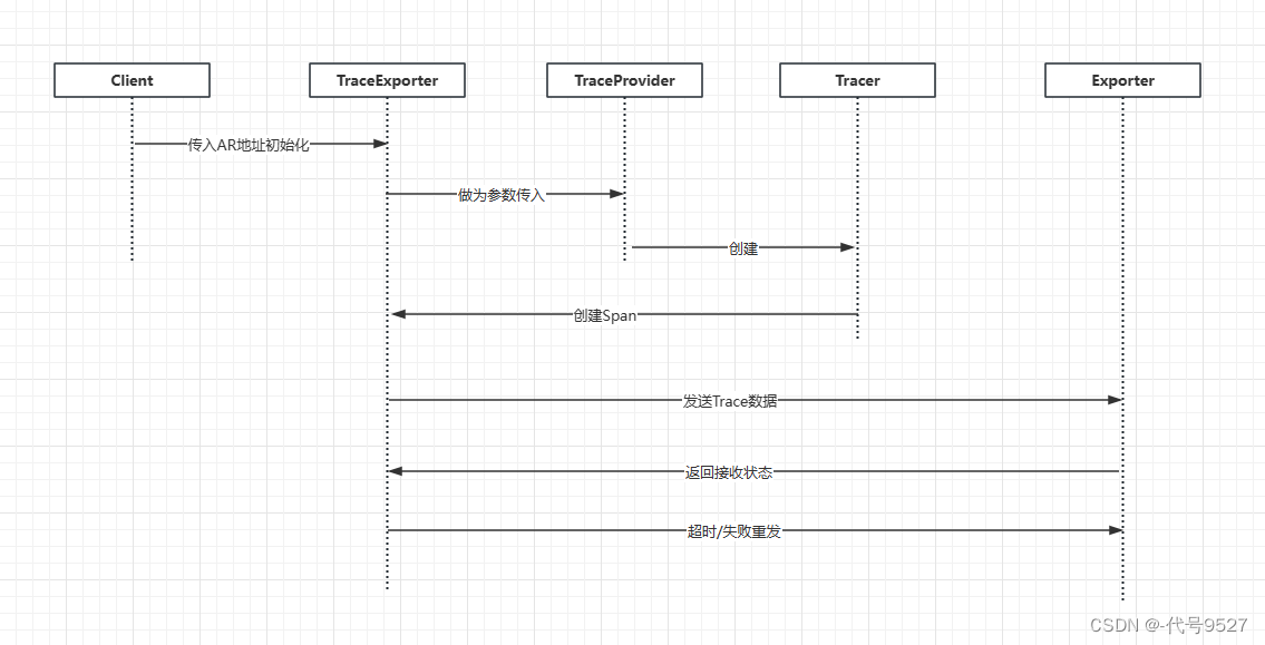
SpringCloud集成OpenTelemetry的实现
SpringCloud项目做链路追踪,比较常见的会集成SleuthZipKin来完成,但这次的需求要集成开源框架OpenTelemetry,这里整理下实现过程。相关文章: 【SpringCloud集成SleuthZipkin进行链路追踪】 【OpenTelemetry框架Trace部分整理】 …...

Python爬取IP归属地信息及各个地区天气信息
一、实现样式 二、核心点 1、语言:Python、HTML,CSS 2、python web框架 Flask 3、三方库:requests、xpath 4、爬取网站:https://ip138.com/ 5、文档结构 三、代码 ipquery.py import requests from lxml import etree # 请求…...
RedLock + Redisson
目录 2.9 RedLock2.9.1 上述实现的分布式锁在集群状态下失效的原因2.9.2 解决方式-RedLock 2.10 redisson中的分布式锁2.10.0 redisson简介以及简单使用简单使用redisson中的锁Redisson常用配置 2.10.1 Redisson可重入锁实现原理2.10.2 公平锁(Fair Lock)…...
计算机视觉:卷积层的参数量是多少?
本文重点 卷积核的参数量是卷积神经网络中一个重要的概念,它决定了网络的复杂度和计算量。在深度学习中,卷积操作是一种常用的操作,用于提取图像、语音等数据中的特征。卷积神经网络的优势点在于稀疏连接和权值共享,这使得卷积核的参数相较于传统的神经网络要少很多。 举例…...
Docker 容器基础操作
Docker容器基础操作 容器(container)是Docker镜像的运行实例,类似于可执行文件与进程的关系,Docker是容器引擎,相当于系统平台。 容器的生命周期 容器的基础操作(以 tomcat8.0 为例) # 拉取tomcat8.0镜像 [root@tudou tudou]# docker pull tomcat:8.0 8.0: Pulling f…...

【Vue3+Ts+Vite】配置滚动条样式
一、先看效果 二、直接上代码 <template><div class"main-container"><h1 v-for"index in 50" :key"index">这是home页面</h1></div> </template> <style lang"scss" scoped> .main-conta…...

GitHub中文界面转换指南:3步打造专属中文GitHub环境
GitHub中文界面转换指南:3步打造专属中文GitHub环境 【免费下载链接】github-chinese GitHub 汉化插件,GitHub 中文化界面。 (GitHub Translation To Chinese) 项目地址: https://gitcode.com/gh_mirrors/gi/github-chinese 当我们第一次接触GitH…...

java springboot-vue加油站管理系统的设计与实现
目录同行可拿货,招校园代理 ,本人源头供货商项目背景技术架构核心功能模块系统特色部署方式应用场景项目技术支持源码获取详细视频演示 :同行可合作点击我获取源码->->进我个人主页-->获取博主联系方式同行可拿货,招校园代理 ,本人源头供货商 项目背景 加…...

油雾净化设备哪家技术更专业
在机械加工、五金锻造、热处理等工业生产场景中,机床切削、乳化液喷淋、高温加工会持续产生大量工业油雾。悬浮在车间内的油雾不仅会腐蚀生产设备、污染生产环境,还会刺激人体呼吸道,危害操作人员身体健康,同时超标排放还会违反环…...
返回False)
保姆级排查指南:PyTorch装完CUDA不认账?手把手教你搞定torch.cuda.is_available()返回False
保姆级排查指南:PyTorch装完CUDA不认账?手把手教你搞定torch.cuda.is_available()返回False 刚装好PyTorch准备大展拳脚,结果torch.cuda.is_available()无情地返回False?这种挫败感我太懂了。作为过来人,我整理了这份…...
:Handle——谁占着不放?句柄泄漏排查、强制解锁与检索技巧)
《Sysinternals实战指南》进程和诊断工具学习笔记(8.24):Handle——谁占着不放?句柄泄漏排查、强制解锁与检索技巧
🔥个人主页:杨利杰YJlio❄️个人专栏:《Sysinternals实战教程》《Windows PowerShell 实战》《WINDOWS教程》《IOS教程》《微信助手》《锤子助手》 《Python》 《Kali Linux》 《那些年未解决的Windows疑难杂症》🌟 让复杂的事情更…...

Aeneas终极指南:3步搞定音频文本自动对齐,准确率超95%
Aeneas终极指南:3步搞定音频文本自动对齐,准确率超95% 【免费下载链接】aeneas aeneas is a Python/C library and a set of tools to automagically synchronize audio and text (aka forced alignment) 项目地址: https://gitcode.com/gh_mirrors/ae…...

AssetStudio v0.16.5深度解析:Unity资源解包原理与工程化实践
1. 为什么你还在手动解包Unity游戏资源?AssetStudio不是“点开即用”的万能钥匙AssetStudio这个名字,听上去像某个高端建模插件,或者Unity官方出的资源管理器——其实它既不是Unity原生工具,也不带任何图形化向导。它是个开源、无…...

AssetStudio深度解析:Unity资源提取原理与跨版本兼容实践
1. 这不是个“点开即用”的工具,而是一把需要校准的Unity资源解剖刀AssetStudio这个名字听起来像某个轻量级小工具,但实际用过的人很快会意识到:它根本不是拿来就跑的“一键提取器”,而是一套需要你亲手调参、理解Unity底层序列化…...

工具调用优化:减少API延迟对Agent性能的影响
《工具调用优化全指南:彻底解决API延迟拖累大模型Agent性能的痛点》 副标题:从原理到落地,覆盖缓存、并行、调度、轻量化改造全链路可复现方案 第一部分:引言与基础 1.1 摘要/引言 你有没有遇到过这种场景:辛辛苦苦开发的智能Agent功能非常强大,能查订单、搜资料、算数…...

JMeter断言实战:从误配到分层校验的避坑指南
1. 为什么断言不是“加个检查框”就完事了?很多人第一次在 JMeter 里点开“添加 → 断言 → 响应断言”,填上“包含文本:success”,跑完看绿色小勾就以为接口测试闭环了。我带过三届测试团队,新同事交来的脚本里&#…...