GEO生信数据挖掘(九)肺结核数据-差异分析-WGCNA分析(900行代码整理注释更新版本)
第六节,我们使用结核病基因数据,做了一个数据预处理的实操案例。例子中结核类型,包括结核,潜隐进展,对照和潜隐,四个类别。第七节延续上个数据,进行了差异分析。 第八节对差异基因进行富集分析。本节进行WGCNA分析。
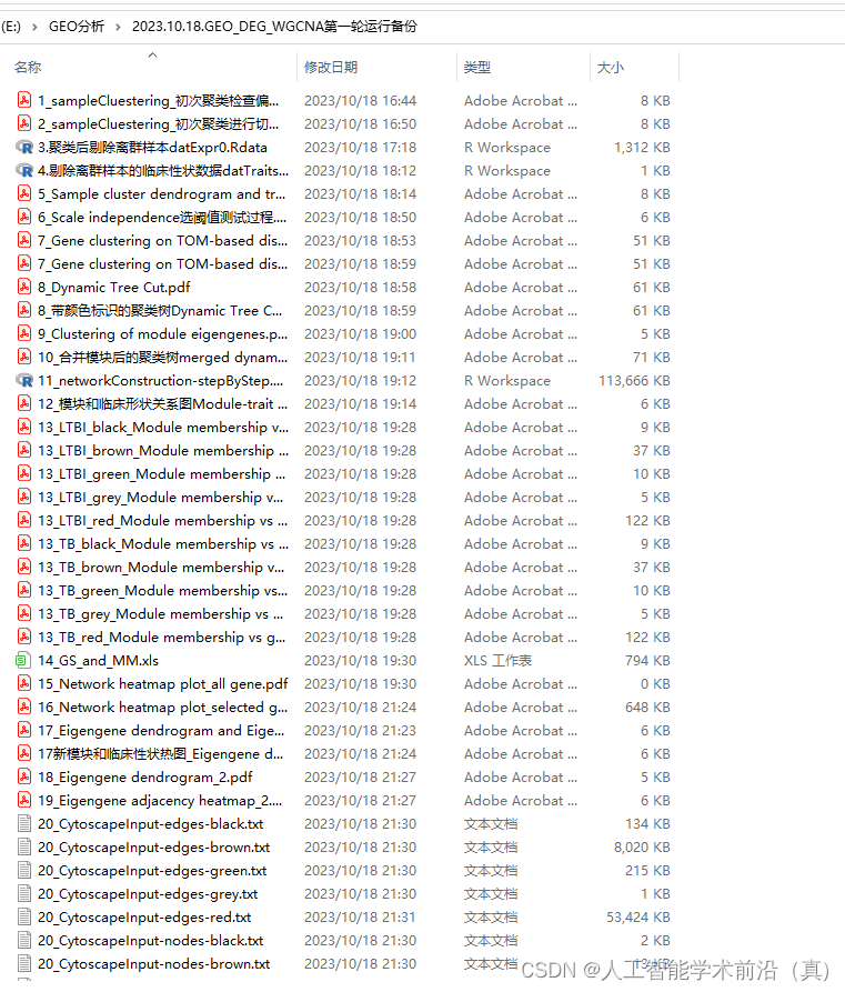
WGCNA分析 分段代码(附运行效果图)请查看上节
运行后效果
rm(list = ls()) ######清除环境数据#============================================================================
#======================================================================
#+========step0数据预处理和检查,已经做过step0==========================
#+========================================
#+=============================
"""
##############设置工作路径###################
workingDir = "C:/Users/Desktop/GSE152532"############工作路径,可以修改,可以设置为数据存放路径
setwd(workingDir)
getwd()################载入R包########################
library(WGCNA)
library(data.table)#############################导入数据##########################
# The following setting is important, do not omit.
options(stringsAsFactors = FALSE)
#Read in the female liver data set
fpkm = fread("Gene_expression.csv",header=T)##############数据文件名,根据实际修改,如果工作路径不是实际数据路径,需要添加正确的数据路径
# Take a quick look at what is in the data set
dim(fpkm)
names(fpkm)####################导入平台数据##########################
library(idmap2)
ids=get_soft_IDs('GPL10558')
head(ids)#####################将探针ID改为基因ID##########################
fpkm<-merge(fpkm,ids,by='ID')#merge()函数将dat1的探针id与芯片平台探针id相匹配,合并到dat1
library(limma)
fpkm<-avereps(fpkm[,-c(1,99)],ID=fpkm$symbol)#多个探针检测一个基因,合并一起,取其平均值
fpkm<-as.data.frame(fpkm)#将矩阵转换为表格
write.table(fpkm, file="FPKM_genesymbol.csv",row.names=T, col.names=T,quote=FALSE,sep=",")
###结束后查看文件,进行修改!!!# 加载自己的数据# load( "group_data_TB_LTBI.Rdata")load("exprSet_clean_mean_filter_log1.RData")  #exprSet_cleanload( "dataset_TB_LTBI.Rdata")
exprSet_clean = dataset_TB_LTBI
gene_var <- apply(exprSet_clean, 1, var)##### 计算基因的方差
keep_genes <- gene_var >= quantile(gene_var, 0.75)##### 筛选方差较大的基因,选择方差前25%的基因
exprSet_clean <- exprSet_clean[keep_genes,]##### 保留筛选后的基因
dim(exprSet_clean)
save (exprSet_clean,file="方差前25per_TB_LTBI.Rdata")#######################基于方差筛选基因#################################
fpkm_var <- read.csv("FPKM_genesymbol.csv", header = TRUE, row.names = 1)##### 读入表达矩阵,矩阵的行是基因,列是样本
gene_var <- apply(fpkm_var, 1, var)##### 计算基因的方差
keep_genes <- gene_var >= quantile(gene_var, 0.75)##### 筛选方差较大的基因,选择方差前25%的基因
fpkm_var <- fpkm_var[keep_genes,]##### 保留筛选后的基因write.table(fpkm_var, file="FPKM_var.csv",row.names=T, col.names=T,quote=FALSE,sep=",")
###结束后查看文件,进行修改!!!##################重新载入数据########################
# The following setting is important, do not omit.
options(stringsAsFactors = FALSE)
#Read in the female liver data set
fpkm = fread("FPKM_var_filter.csv",header=T)##############数据文件名,根据实际修改,如果工作路径不是实际数据路径,需要添加正确的数据路径
# Take a quick look at what is in the data set
dim(fpkm)
names(fpkm)datExpr0 = as.data.frame(t(fpkm[,-1]))
names(datExpr0) = fpkm$ID;##########如果第一行是ID命名,就写成fpkm$ID
rownames(datExpr0) = names(fpkm[,-1])##################check missing value and filter ####################
load("方差前25per_TB_LTBI.Rdata")
datExpr0  = exprSet_clean##check missing value
library(WGCNA)
gsg = goodSamplesGenes(datExpr0, verbose = 3)
gsg$allOKif (!gsg$allOK)
{# Optionally, print the gene and sample names that were removed:if (sum(!gsg$goodGenes)>0)printFlush(paste("Removing genes:", paste(names(datExpr0)[!gsg$goodGenes], collapse = ", ")))if (sum(!gsg$goodSamples)>0)printFlush(paste("Removing samples:", paste(rownames(datExpr0)[!gsg$goodSamples], collapse = ", ")))# Remove the offending genes and samples from the data:datExpr0 = datExpr0[gsg$goodSamples, gsg$goodGenes]
}##filter
#meanFPKM=0.5  ####过滤标准,可以修改
#n=nrow(datExpr0)
#datExpr0[n+1,]=apply(datExpr0[c(1:nrow(datExpr0)),],2,mean)
#datExpr0=datExpr0[1:n,datExpr0[n+1,] > meanFPKM]  # for meanFpkm in row n+1 and it must be above what you set--select meanFpkm>opt$meanFpkm(by rp)filtered_fpkm=t(datExpr0)  #行 样本 列 基因
filtered_fpkm=data.frame(rownames(filtered_fpkm),filtered_fpkm)
names(filtered_fpkm)[1]="sample"
write.table(filtered_fpkm, file="FPKM_filter.csv",row.names=F, col.names=T,quote=FALSE,sep="\t")"""#&&&&&&&&&&&&&&&&&&&&&&&&&&&&&&&&&&&&&&&&&&&&&&&&&&&&&&&&&&&&&&&&&&&&&&&&&&&&&&&&&&&&
#+&&&&&&&&&&&&&&&&&&加载数据&&&&&&&&&&&&&&&&&&&&&&&&&&&&&&&&&&&&&&&&&&&&&&&&&&&&&&&&&
#++++++++++++++++++++++++++++++++++++++++++++++++++++++++++++
load('DEG_TB_LTBI_step13.Rdata')  # DEG,res,all_diff,limma_clean_res,dataset_TB_LTBI_DEG,
#++++++++++++++++++++++++++++++++++++++++++++++++++++++++++++
#+&&&&&&&&&&&&&&&&&&加载数据&&&&&&&&&&&&&&&&&&&&&&&&&&&&&&&&&&&&&&&&&&&&&&&&&&&&&&&&&
#&&&&&&&&&&&&&&&&&&&&&&&&&&&&&&&&&&&&&&&&&&&&&&&&&&&&&&&&&&&&&&&&&&&&&&&&&&&&&&&&&&&&library(WGCNA)
#读取目录名称,方便复制粘贴
dir()#============================================================================
#======================================================================
#+========step1样品聚类step1=================================
#+========================================
#+=============================################################样品聚类####################
#这里行是样品名,列为基因名,做转置处理
datExpr = t(dataset_TB_LTBI_DEG)
#初次聚类
sampleTree = hclust(dist(datExpr), method = "average")
# Plot the sample tree: Open a graphic output window of size 20 by 15 inches
# The user should change the dimensions if the window is too large or too small.
#设置绘图窗口
sizeGrWindow(12,9)
pdf(file='1_sampleCluestering_初次聚类检查偏离样本.pdf',width = 12,height = 9)
par(cex=0.6)
par(mar=c(0,4,2,0))
plot(sampleTree, main = "Sample clustering to detect outliers", sub="", xlab="", cex.lab = 1.5,cex.axis = 1.5, cex.main = 2)dev.off()#============================================================================
#======================================================================
#+========step2切割离群样本=================================
#+========================================
#+=============================pdf(file='2_sampleCluestering_初次聚类进行切割删除样本.pdf',width = 12,height = 9)
par(cex=0.6)
par(mar=c(0,4,2,0))
plot(sampleTree, main = "Sample clustering to detect outliers ", sub="", xlab="", cex.lab = 1.5,cex.axis = 1.5, cex.main = 2)### 测试画线,可以多次尝试
##############剪切高度问题,这个根据实际设置后可用
abline(h = 87, col = "red")##剪切高度不确定,故无红线
dev.off()### Determine cluster under the line
clust = cutreeStatic(sampleTree, cutHeight = 87, minSize = 10)
table(clust)
#clust
#0  1  2
#5 57 40
#由于本人案例,一刀切出三段,需要保留两段,用了’或‘逻辑运算符号
### 需要保留哪个,就传如要保留clust编号
keepSamples = (clust==1|clust==2)
#剔除离群样本
datExpr0 = datExpr[keepSamples, ]
#观察新表达矩阵
dim(datExpr0) #[1]   97 2813#&&&&&&&&&&&&&&&&&&&&&&&&&&&&&&&&&&&&&&&&&&&&&&&&&&&&&&&&&&&&
#+&&&&&&&&&&&&&&&&&&数据保存&&&&&&&&&&&&&&&&&&&&&&&&&&&&&&&&&
#++++++++++++++++++++++++++++++++++++++++++++++++++++++++++++
save(datExpr0,file='3.聚类后剔除离群样本datExpr0.Rdata')#++++++++++++++++++++++++++++++++++++++++++++++++++++++++++++
#+&&&&&&&&&&&&&&&&&&数据保存&&&&&&&&&&&&&&&&&&&&&&&&&&&&&&&&&
#&&&&&&&&&&&&&&&&&&&&&&&&&&&&&&&&&&&&&&&&&&&&&&&&&&&&&&&&&&&&load('datExpr0_cluster_filter.Rdata')#============================================================================
#======================================================================
#+========step3临床性状数据整理,与新表达矩阵保持一致=================================
#+========================================
#+=============================#加载自己的临床性状数据
load('design_TB_LTBI.Rdata')
traitData=designdim(traitData)# Form a data frame analogous to expression data that will hold the clinical traits.
fpkmSamples = rownames(datExpr0)
traitSamples =rownames(traitData)
#匹配样本名称,性状数据与表达数据保证一致
traitRows = match(fpkmSamples, traitSamples)
datTraits = traitData[traitRows,]
rownames(datTraits)
collectGarbage()#&&&&&&&&&&&&&&&&&&&&&&&&&&&&&&&&&&&&&&&&&&&&&&&&&&&&&&&&&&&&
#+&&&&&&&&&&&&&&&&&&数据保存&&&&&&&&&&&&&&&&&&&&&&&&&&&&&&&&&
#++++++++++++++++++++++++++++++++++++++++++++++++++++++++++++
save(datTraits,file='4.剔除离群样本的临床性状数据datTraits.Rdata')#++++++++++++++++++++++++++++++++++++++++++++++++++++++++++++
#+&&&&&&&&&&&&&&&&&&数据保存&&&&&&&&&&&&&&&&&&&&&&&&&&&&&&&&&
#&&&&&&&&&&&&&&&&&&&&&&&&&&&&&&&&&&&&&&&&&&&&&&&&&&&&&&&&&&&&#============================================================================
#======================================================================
#+========step4 增加临床性状数据后再次聚类=======================
#+========================================
#+=============================
# Re-cluster samples
sampleTree2 = hclust(dist(datExpr0), method = "average")
# Convert traits to a color representation: white means low, red means high, grey means missing entry
traitColors = numbers2colors(datTraits, signed = FALSE)
# Plot the sample dendrogram and the colors underneath.#sizeGrWindow(20,20)pdf(file="5_Sample cluster dendrogram and trait heatmap.pdf",width=12,height=12)
plotDendroAndColors(sampleTree2, traitColors,groupLabels = names(datTraits),main = "Sample dendrogram and trait heatmap")#Error in .plotOrderedColorSubplot(order = order, colors = colors, rowLabels = rowLabels,  :
#                                    Length of colors vector not compatible with number of objects in 'order'.dev.off()#============================================================================
#======================================================================
#+========step5 构建WGCNA网络=======================
#+========================================
#+=============================# Allow multi-threading within WGCNA. At present this call is necessary.
# Any error here may be ignored but you may want to update WGCNA if you see one.
# Caution: skip this line if you run RStudio or other third-party R environments.
# See note above.
#检查环境,能开几个线程
enableWGCNAThreads()# Choose a set of soft-thresholding powers
#设置阈值范围,WGCNA是无标度网络(scale free),节点连结数服从幂次定律分布。(连接数越多核心节点越少)
powers = c(1:15)# Call the network topology analysis function
#网络拓扑分析
sft = pickSoftThreshold(datExpr0, powerVector = powers, verbose = 5)# Plot the results:
sizeGrWindow(15, 9)
pdf(file="6_Scale independence选阈值测试过程.pdf",width=9,height=5)
#pdf(file="Rplot03.pdf",width=9,height=5)
par(mfrow = c(1,2))
cex1 = 0.9
# Scale-free topology fit index as a function of the soft-thresholding power
#无标度拓扑拟合指标作为软阈值能力的函数,根据下图结果,挑选合适阈值
plot(sft$fitIndices[,1], -sign(sft$fitIndices[,3])*sft$fitIndices[,2],xlab="Soft Threshold (power)",ylab="Scale Free Topology Model Fit,signed R^2",type="n",main = paste("Scale independence"));
text(sft$fitIndices[,1], -sign(sft$fitIndices[,3])*sft$fitIndices[,2],labels=powers,cex=cex1,col="red");
# this line corresponds to using an R^2 cut-off of h
abline(h=0.90,col="red")
# Mean connectivity as a function of the soft-thresholding power
plot(sft$fitIndices[,1], sft$fitIndices[,5],xlab="Soft Threshold (power)",ylab="Mean Connectivity", type="n",main = paste("Mean connectivity"))
text(sft$fitIndices[,1], sft$fitIndices[,5], labels=powers, cex=cex1,col="red")
dev.off()######chose the softPower
#选择阈值
softPower =sft$powerEstimate
adjacency = adjacency(datExpr0, power = softPower)##### Turn adjacency into topological overlap
#将邻接转换为拓扑重叠
TOM = TOMsimilarity(adjacency);
dissTOM = 1-TOM# Call the hierarchical clustering function
#无标度网络阈值参数确定后,调用分层聚类函数
#基于TOM的不相似性基因聚类
geneTree = hclust(as.dist(dissTOM), method = "average");
# Plot the resulting clustering tree (dendrogram)#sizeGrWindow(12,9)
pdf(file="7_Gene clustering on TOM-based dissimilarity基因聚类图.pdf",width=12,height=9)
plot(geneTree, xlab="", sub="", main = "Gene clustering on TOM-based dissimilarity",labels = FALSE, hang = 0.04)
dev.off()#聚类模块,最小的基因数量
# We like large modules, so we set the minimum module size relatively high:
minModuleSize = 30# Module identification using dynamic tree cut:
#使用dynamic tree cut进行模块识别
dynamicMods = cutreeDynamic(dendro = geneTree, distM = dissTOM,deepSplit = 2, pamRespectsDendro = FALSE,minClusterSize = minModuleSize);
table(dynamicMods)# Convert numeric lables into colors
#给不同模块分配颜色
dynamicColors = labels2colors(dynamicMods)
table(dynamicColors)
# Plot the dendrogram and colors underneath
#sizeGrWindow(8,6)
pdf(file="8_带颜色标识的聚类树Dynamic Tree Cut.pdf",width=8,height=6)
plotDendroAndColors(geneTree, dynamicColors, "Dynamic Tree Cut",dendroLabels = FALSE, hang = 0.03,addGuide = TRUE, guideHang = 0.05,main = "Gene dendrogram and module colors")
dev.off()# Calculate eigengenes
MEList = moduleEigengenes(datExpr0, colors = dynamicColors)
MEs = MEList$eigengenes
# Calculate dissimilarity of module eigengenes
MEDiss = 1-cor(MEs);
# Cluster module eigengenes
METree = hclust(as.dist(MEDiss), method = "average")
# Plot the result
#sizeGrWindow(7, 6)
pdf(file="9_Clustering of module eigengenes.pdf",width=7,height=6)
plot(METree, main = "Clustering of module eigengenes",xlab = "", sub = "")
MEDissThres = 0.25######剪切高度可修改
# Plot the cut line into the dendrogram
abline(h=MEDissThres, col = "red")
dev.off()# Call an automatic merging function
#根据前面设置的剪切高度,对模块进行合并
merge = mergeCloseModules(datExpr0, dynamicColors, cutHeight = MEDissThres, verbose = 3)
# The merged module colors
mergedColors = merge$colors
# Eigengenes of the new merged modules:
mergedMEs = merge$newMEs#sizeGrWindow(12, 9)
pdf(file="10_合并模块后的聚类树merged dynamic.pdf", width = 9, height = 6)
plotDendroAndColors(geneTree, cbind(dynamicColors, mergedColors),c("Dynamic Tree Cut", "Merged dynamic"),dendroLabels = FALSE, hang = 0.03,addGuide = TRUE, guideHang = 0.05)
dev.off()# Rename to moduleColors
moduleColors = mergedColors
# Construct numerical labels corresponding to the colors
#构建相应颜色的数字标签
colorOrder = c("grey", standardColors(50))
moduleLabels = match(moduleColors, colorOrder)-1
MEs = mergedMEs# Save module colors and labels for use in subsequent parts
#&&&&&&&&&&&&&&&&&&&&&&&&&&&&&&&&&&&&&&&&&&&&&&&&&&&&&&&&&&&&
#+&&&&&&&&&&&&&&&&&&数据保存&&&&&&&&&&&&&&&&&&&&&&&&&&&&&&&&&
#++++++++++++++++++++++++++++++++++++++++++++++++++++++++++++
save(datExpr0,datTraits,MEs, TOM, dissTOM,  moduleLabels, moduleColors, geneTree, sft, file = "11_networkConstruction-stepByStep.RData")
#++++++++++++++++++++++++++++++++++++++++++++++++++++++++++++
#+&&&&&&&&&&&&&&&&&&数据保存&&&&&&&&&&&&&&&&&&&&&&&&&&&&&&&&&
#&&&&&&&&&&&&&&&&&&&&&&&&&&&&&&&&&&&&&&&&&&&&&&&&&&&&&&&&&&&&load("11_networkConstruction-stepByStep.RData")#=====================================================================================
#===============================================================================
#+========step6 计算模块和临床性状相关系数(核心挑选色块)==============
#+========================================
#+=============================
##############################relate modules to external clinical triats# Define numbers of genes and samples
nGenes = ncol(datExpr0)
nSamples = nrow(datExpr0)#可以修改参数 p值pvalue 更换
moduleTraitCor = cor(MEs, datTraits, use = "p")
moduleTraitPvalue = corPvalueStudent(moduleTraitCor, nSamples)#sizeGrWindow(10,6)
pdf(file="12_模块和临床形状关系图Module-trait relationships.pdf",width=10,height=6)
# Will display correlations and their p-values
textMatrix = paste(signif(moduleTraitCor, 2), "\n(",signif(moduleTraitPvalue, 1), ")", sep = "")dim(textMatrix) = dim(moduleTraitCor)
par(mar = c(6, 8.5, 3, 3))# Display the correlation values within a heatmap plot #修改性状类型 data.frame
labeledHeatmap(Matrix = moduleTraitCor,xLabels = names(data.frame(datTraits)),yLabels = names(MEs),ySymbols = names(MEs),colorLabels = FALSE,colors = greenWhiteRed(50),textMatrix = textMatrix,setStdMargins = FALSE,cex.text = 0.5,zlim = c(-1,1),main = paste("Module-trait relationships"))
dev.off()#色块 red相关度 0.75#=====================================================================================
#===============================================================================
#+========step7 定义包含所有datTraits列的可变权重(MM and GS)==============
#+========================================
#+=============================#定义包含所有datTraits列的可变权重######## Define variable weight containing all column of datTraits###MM(gene Module Membership) and GS(gene Trait Significance)# names (colors) of the modules
modNames = substring(names(MEs), 3)geneModuleMembership = as.data.frame(cor(datExpr0, MEs, use = "p"))
MMPvalue = as.data.frame(corPvalueStudent(as.matrix(geneModuleMembership), nSamples))names(geneModuleMembership) = paste("MM", modNames, sep="")
names(MMPvalue) = paste("p.MM", modNames, sep="")#names of those trait
traitNames=names(data.frame(datTraits))
class(datTraits)geneTraitSignificance = as.data.frame(cor(datExpr0, datTraits, use = "p"))
GSPvalue = as.data.frame(corPvalueStudent(as.matrix(geneTraitSignificance), nSamples))names(geneTraitSignificance) = paste("GS.", traitNames, sep="")
names(GSPvalue) = paste("p.GS.", traitNames, sep="")####plot MM vs GS for each trait vs each module##########example:royalblue and CK
module="red"
column = match(module, modNames)
moduleGenes = moduleColors==moduletrait="TB"
traitColumn=match(trait,traitNames)sizeGrWindow(7, 7)#par(mfrow = c(1,1))
verboseScatterplot(abs(geneModuleMembership[moduleGenes, column]),
abs(geneTraitSignificance[moduleGenes, traitColumn]),
xlab = paste("Module Membership in", module, "module"),
ylab = paste("Gene significance for ",trait),
main = paste("Module membership vs. gene significance\n"),
cex.main = 1.2, cex.lab = 1.2, cex.axis = 1.2, col = module)
######for (trait in traitNames){traitColumn=match(trait,traitNames)for (module in modNames){column = match(module, modNames)moduleGenes = moduleColors==moduleif (nrow(geneModuleMembership[moduleGenes,]) > 1){####进行这部分计算必须每个模块内基因数量大于2,由于前面设置了最小数量是30,这里可以不做这个判断,但是grey有可能会出现1个gene,它会导致代码运行的时候中断,故设置这一步#sizeGrWindow(7, 7)pdf(file=paste("13_", trait, "_", module,"_Module membership vs gene significance.pdf",sep=""),width=7,height=7)par(mfrow = c(1,1))verboseScatterplot(abs(geneModuleMembership[moduleGenes, column]),abs(geneTraitSignificance[moduleGenes, traitColumn]),xlab = paste("Module Membership in", module, "module"),ylab = paste("Gene significance for ",trait),main = paste("Module membership vs. gene significance\n"),cex.main = 1.2, cex.lab = 1.2, cex.axis = 1.2, col = module)dev.off()}}
}#####
names(datExpr0)
probes = names(data.frame(datExpr0))#=====================================================================================
#===============================================================================
#+========step8 导出计算完毕的(MM and GS)==============
#+========================================
#+=============================
#################export GS and MM############### geneInfo0 = data.frame(probes= probes,moduleColor = moduleColors)for (Tra in 1:ncol(geneTraitSignificance))
{oldNames = names(geneInfo0)geneInfo0 = data.frame(geneInfo0, geneTraitSignificance[,Tra],GSPvalue[, Tra])names(geneInfo0) = c(oldNames,names(geneTraitSignificance)[Tra],names(GSPvalue)[Tra])
}for (mod in 1:ncol(geneModuleMembership))
{oldNames = names(geneInfo0)geneInfo0 = data.frame(geneInfo0, geneModuleMembership[,mod],MMPvalue[, mod])names(geneInfo0) = c(oldNames,names(geneModuleMembership)[mod],names(MMPvalue)[mod])
}
geneOrder =order(geneInfo0$moduleColor)
geneInfo = geneInfo0[geneOrder, ]write.table(geneInfo, file = "14_GS_and_MM.xls",sep="\t",row.names=F)#=====================================================================================
#===============================================================================
#+========step9 基因网络热图进行可视化(非常耗费内存资源)==============
#+========================================
#+=============================nGenes = ncol(datExpr0)
nSamples = nrow(datExpr0)# Transform dissTOM with a power to make moderately strong connections more visible in the heatmap
plotTOM = dissTOM^7
# Set diagonal to NA for a nicer plot
diag(plotTOM) = NA# Call the plot functionsizeGrWindow(9,9)  #这个耗电脑内存
pdf(file="15_所有基因数量太多Network heatmap plot_all gene.pdf",width=9, height=9)
TOMplot(plotTOM, geneTree, moduleColors, main = "Network heatmap plot, all genes")
dev.off()nSelect = 400
# For reproducibility, we set the random seed
set.seed(10)
select = sample(nGenes, size = nSelect)
selectTOM = dissTOM[select, select]
# There's no simple way of restricting a clustering tree to a subset of genes, so we must re-cluster.
selectTree = hclust(as.dist(selectTOM), method = "average")
selectColors = moduleColors[select]# Open a graphical window
#sizeGrWindow(9,9)
# Taking the dissimilarity to a power, say 10, makes the plot more informative by effectively changing
# the color palette; setting the diagonal to NA also improves the clarity of the plot
plotDiss = selectTOM^7
diag(plotDiss) = NApdf(file="16_400个基因试试Network heatmap plot_selected genes.pdf",width=9, height=9)
TOMplot(plotDiss, selectTree, selectColors, main = "Network heatmap plot, selected genes")
dev.off()#=====================================================================================
#===============================================================================
#+========step10 新模块和临床性状热图 合并和拆分两个版本==============
#+========================================
#+=============================#sizeGrWindow(5,7.5)
pdf(file="17新模块和临床性状热图_Eigengene dendrogram and Eigengene adjacency heatmap.pdf", width=5, height=7.5)
par(cex = 0.9)
plotEigengeneNetworks(MEs, "", marDendro = c(0,4,1,2), marHeatmap = c(3,4,1,2), cex.lab = 0.8, xLabelsAngle= 90)
dev.off()#or devide into two parts
# Plot the dendrogram
#sizeGrWindow(6,6);
pdf(file="18_Eigengene dendrogram_2.pdf",width=6, height=6)
par(cex = 1.0)
plotEigengeneNetworks(MEs, "Eigengene dendrogram", marDendro = c(0,4,2,0), plotHeatmaps = FALSE)
dev.off()pdf(file="19_Eigengene adjacency heatmap_2.pdf",width=6, height=6)
# Plot the heatmap matrix (note: this plot will overwrite the dendrogram plot)
par(cex = 1.0)
plotEigengeneNetworks(MEs, "Eigengene adjacency heatmap", marHeatmap = c(3,4,2,2), plotDendrograms = FALSE, xLabelsAngle = 90)
dev.off()###########################Exporting to Cytoscape all one by one ###########################=====================================================================================
#===============================================================================
#+========step11 导出每个模块的边和节点关系(Cytoscape 绘图所需)==============
#+========================================
#+=============================# Select each module
'''
Error in exportNetworkToCytoscape(modTOM, edgeFile = paste("CytoscapeInput-edges-",  : Cannot determine node names: nodeNames is NULL and adjMat has no dimnames.datExpr0 格式需要dataframe
'''
modules =module  #module="red"
for (mod in 1:nrow(table(moduleColors)))
{modules = names(table(moduleColors))[mod]# Select module probesprobes = names(data.frame(datExpr0))  # inModule = (moduleColors == modules)modProbes = probes[inModule]modGenes = modProbes# Select the corresponding Topological OverlapmodTOM = TOM[inModule, inModule]dimnames(modTOM) = list(modProbes, modProbes)# Export the network into edge and node list files Cytoscape can readcyt = exportNetworkToCytoscape(modTOM,edgeFile = paste("20_CytoscapeInput-edges-", modules , ".txt", sep=""),nodeFile = paste("20_CytoscapeInput-nodes-", modules, ".txt", sep=""),weighted = TRUE,threshold = 0.02,nodeNames = modProbes,altNodeNames = modGenes,nodeAttr = moduleColors[inModule])
}
WGCNA关系网络的构建完毕,绘图找核心基因,Cytoscape 到底怎么玩?
相关文章:
GEO生信数据挖掘(九)肺结核数据-差异分析-WGCNA分析(900行代码整理注释更新版本)
第六节,我们使用结核病基因数据,做了一个数据预处理的实操案例。例子中结核类型,包括结核,潜隐进展,对照和潜隐,四个类别。第七节延续上个数据,进行了差异分析。 第八节对差异基因进行富集分析。…...

二进制明文字符串加密:实现原理
二进制明文字符串加密:实现原理 背景 这里就不多做解释了,明文字符串暴露就是最好的逆向分析指引。无论是恶意攻击样本还是有一定安全需求的组件,直接暴露程序中的明文字符串会大幅降低外部的分析成本。所以需要在编译出的二进制中隐藏字符串。不过需要…...

免费SSL证书:JoySSL让您的网站更安全
在今天的数字化时代,保护网站和用户信息的安全至关重要。SSL(Secure Sockets Layer)证书通过加密网站与用户之间的通信,确保数据传输的安全性。让您拥有一个SSL加密的网站是至关重要的,但您可能会担心高昂的费用。不过…...

JavaPTA练习题 7-3 打印99乘法表
打印99乘法表 输入样例: 不需要输入 输出样例: 在这里给出相应的输出。要求:99乘法表中,每个表达式的乘法结果长度为3。 1x11 2x12 2x24 3x13 3x26 3x39 4x14 4x28 4x312 4x416 5x15 5x210 5x315 5x420 5x525 6x16 6x212 6x318 6x424…...
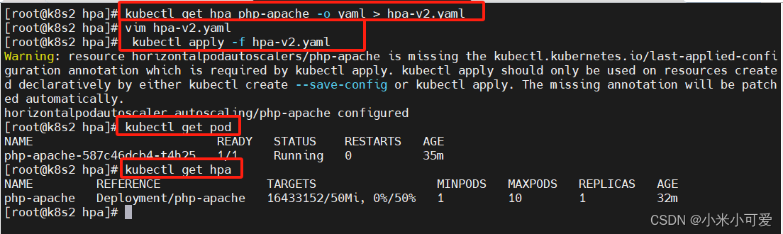
k8s-20 hpa控制器
hpa可通过metrics-server所提供pod的cpu 或者内存的负载情况,从而动态拉伸控制器的副本数,从而达到后端的自动弹缩 官网:https://kubernetes.io/zh-cn/docs/tasks/run-application/horizontal-pod-autoscale-walkthrough/ 上传镜像 压测 po…...
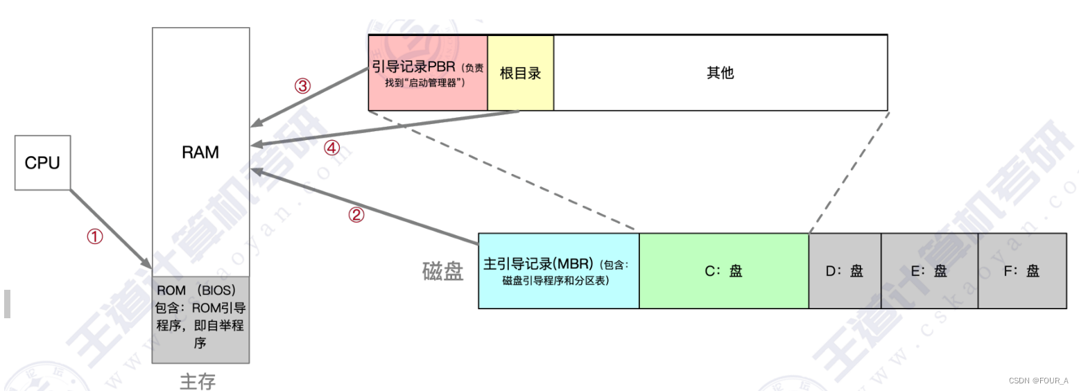
操作系统【OS】操作系统的引导
激活CPU。 激活的CPU读取ROM中的boot程序,将指令寄存器置为BIOS(基本输入输出系统)的第一条指令, 即开始执行BIOS的指令。硬件自检。 启动BIOS程序后,先进行硬件自检,检查硬件是否出现故障。如有故障,主板会发出不同含…...
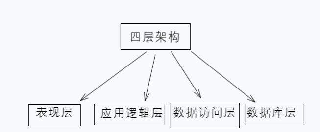
PHP的四层架构
PHP的4层架构是一种软件设计模式,用于将一个PHP应用程序划分为不同的层次,以实现解耦、可扩展和易于维护的代码结构。这个架构通常由以下四个层次组成: 1、 表现层(Presentation Layer): 表现层是与用户直…...
Kafka存取原理与实现分析,打破面试难关
系列文章目录 上手第一关,手把手教你安装kafka与可视化工具kafka-eagle Kafka是什么,以及如何使用SpringBoot对接Kafka 架构必备能力——kafka的选型对比及应用场景 Kafka存取原理与实现分析,打破面试难关 系列文章目录一、主题与分区1. 模型…...

JavaWeb——IDEA相关配置(Tomcat安装)
3、Tomcat 3.1、Tomcat安装 可以在国内一些镜像网站中下载Tomcat,同样也可以在[Tomcat官网](Apache Tomcat - Welcome!)下载 3.2、Tomcat启动和配置 一些文件夹的说明 启动,关闭Tomcat 启动:Tomcat文件夹→bin→startup.bat 关闭&#…...

MySQL:BETWEEN AND操作符的边界
文档原文: expr BETWEEN min AND maxIf expr is greater than or equal to min and expr is less than or equal to max, BETWEEN returns 1, otherwise it returns 0. This is equivalent to the expression (min < expr AND expr < max) if all the argume…...
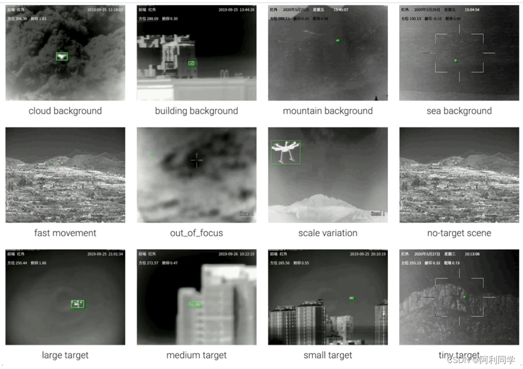
无人机UAV目标检测与跟踪(代码+数据)
前言 近年来,随着无人机的自主性、灵活性和广泛的应用领域,它们在广泛的消费通讯和网络领域迅速发展。无人机应用提供了可能的民用和公共领域应用,其中可以使用单个或多个无人机。与此同时,我们也需要意识到无人机侵入对空域安全…...
Spring中配置文件参数化
目录 一、什么是配置文件参数化 二、配置文件参数化的开发步骤 一、什么是配置文件参数化 配置文件参数化就是将Spring中经常需要修改的字符串信息,转移到一个更小的配置文件中。那么为什么要进行配置文件参数化呢?我们看一个代码 <bean id"co…...
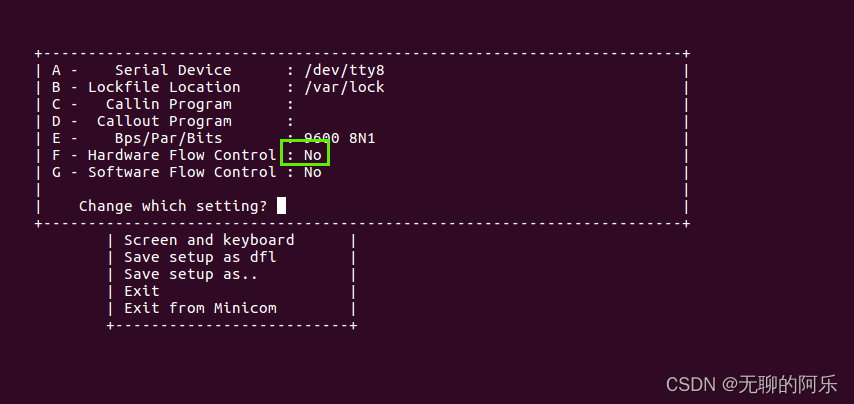
linux minicom 调试串口
1、使用方法 1. 打开终端 2. 输入命令:minicom -D /dev/ttyS0 3. 按下回车键,进入minicom终端界面 4. 在终端界面中发送指令或数据,查看设备返回的数据 5. 按下CtrlA,松开释放,再按下X,退出minicom2、一些…...

#力扣:2651. 计算列车到站时间@FDDLC
2651. 计算列车到站时间 - 力扣(LeetCode) 一、Java class Solution {public int findDelayedArrivalTime(int arrivalTime, int delayedTime) {return (arrivalTimedelayedTime)%24;} }...

小县城蔬菜配送小程序制作全攻略
随着互联网的普及和人们对生活品质要求的提高,越来越多的小县城开始开发蔬菜配送小程序,以满足当地居民对新鲜蔬菜的需求。制作一个小县城蔬菜配送小程序,需要经过以下步骤: 步骤一:登录乔拓云平台 首先,打…...

JavaPTA练习题 7-4 计算给定两数之间的所有奇数之和
本题目要求接收输入的2个整数a和b,然后输出a~b之间的所有奇数之和。 输入格式: 分别用两行输入两个整数a,b 输出格式: 输出a~b之间的所有奇数之和 输入样例: 在这里给出一组输入。例如: 1 30输出样例: 在这里给出相应的输出。例如: …...

基于SSM的大学校医管理系统
基于SSM的大学校医管理系统、学校医院管理系统的设计与实现~ 开发语言:Java数据库:MySQL技术:SpringSpringMVCMyBatisVue工具:IDEA/Ecilpse、Navicat、Maven 系统展示 主页 登录系统 用户界面 管理员界面 摘要 大学校医管理系统…...

【递归、搜索与回溯算法】第一节.初识递归、搜索与回溯算法
作者简介:大家好,我是未央; 博客首页:未央.303 系列专栏:递归、搜索与回溯算法 每日一句:人的一生,可以有所作为的时机只有一次,那就是现在!!!&am…...

第十二届蓝桥杯模拟赛第一期
A填空题 问题描述 如果整数a是整数b的整数倍,则称b是a的约数。 请问,有多少个正整数是2020的约数。 答案提交 这是一道结果填空的题,你只需要算出结果后提交即可。本题的结果为一个整数,在提交答案时只填写这个整数࿰…...

【生成对抗网络】
生成对抗网络(Generative Adversarial Networks,简称GANs)是深度学习领域的一种创新结构,由Ian Goodfellow在2014年首次提出。GANs包括两个深度神经网络——一个生成器和一个判别器,它们通常以对抗的方式进行训练。 以…...

TensorRT安装后验证的几种实用方法:从sample_mnist到PyTorch/TensorFlow模型
TensorRT环境验证全指南:从基础测试到多框架实战 当你完成TensorRT的安装后,最迫切的问题往往是:"我的环境真的装对了吗?"作为NVIDIA推出的高性能深度学习推理引擎,TensorRT的安装验证远比简单的版本检查复杂…...

跨越数字边界的文化守护者:AO3-Mirror-Site开源镜像网络革命
跨越数字边界的文化守护者:AO3-Mirror-Site开源镜像网络革命 【免费下载链接】AO3-Mirror-Site 项目地址: https://gitcode.com/gh_mirrors/ao/AO3-Mirror-Site 当一位中国同人创作者在深夜试图访问AO3却遭遇连接失败,当一位研究者需要引用特定同…...

用STM32的3个GPIO口扩展8路ADC输入?试试74HC4051模拟开关的实战配置
用STM32的3个GPIO口扩展8路ADC输入?74HC4051模拟开关实战指南 在嵌入式开发中,ADC通道不足是个常见痛点。想象一下这样的场景:你的STM32项目需要同时采集8路温度传感器数据,但手头的MCU只有1-2个ADC通道。直接换芯片成本高&#…...

Clawdbot+Qwen3:32B应用案例:如何用AI快速为《论语》《史记》加标点
ClawdbotQwen3:32B应用案例:如何用AI快速为《论语》《史记》加标点 1. 古籍标点处理的痛点与AI解决方案 阅读古籍时最头疼的是什么?对大多数人来说,不是生僻字,不是文言语法,而是那些密密麻麻没有标点的原文。传统古…...

OpenAL32.dll文件丢失找不到怎么办?免费下载方法分享
在使用电脑系统时经常会出现丢失找不到某些文件的情况,由于很多常用软件都是采用 Microsoft Visual Studio 编写的,所以这类软件的运行需要依赖微软Visual C运行库,比如像 QQ、迅雷、Adobe 软件等等,如果没有安装VC运行库或者安装…...

智能修复中的缺陷检测与修补建议
智能修复中的缺陷检测与修补建议 随着人工智能技术的快速发展,智能修复系统在软件开发、工业制造等领域发挥着越来越重要的作用。缺陷检测与修补是智能修复的核心环节,能够帮助开发者快速发现并修复代码或产品中的问题,提高效率并降低成本。…...

Matplotlib与Cartopy的完美结合:只在特定子图上添加海岸线
在数据可视化领域,Matplotlib和Cartopy是两个非常强大的工具。Matplotlib可以用来创建各种图表,而Cartopy则提供了丰富的地理投影和地图绘制功能。最近,我在使用这两个库时遇到一个有趣的问题:如何在一个多子图的图形中,只在特定的子图上添加海岸线,而不是所有的子图。本…...

匈牙利算法
目标:看是否存在一对一映射 应用场景: 假设有n个被试,每个被试有一个功能连接矩阵,然后有一个预测功能连接矩阵,我们想看被试预测的功能连接矩阵是否能够完美匹配自己的真实功能连接矩阵。 1.首先构建真实-预测功能…...

Hadoop 完整入门详解
Apache Hadoop 是 Apache 开源的大数据分布式基础框架,基于廉价普通服务器集群,解决 PB/EB 级海量数据的存储、离线批量计算 问题,是整个大数据生态的基石。灵感源自 Google GFS、MapReduce 论文,Java 开发,名字源于创…...

【深度解析】Cloud Context:给 AI 编码助手装上“代码库 RAG”,彻底解决大型仓库上下文获取难题
摘要 Cloud Context 的核心价值不在“更强模型”,而在“更高效上下文获取”。本文从 RAG、混合检索、AST 分块、增量索引等角度,系统解析它为何能显著提升 AI Coding Agent 在大型代码仓库中的可用性,并给出一套可落地的 Python 实战示例&…...