Lesson11---分类问题
11.1 逻辑回归
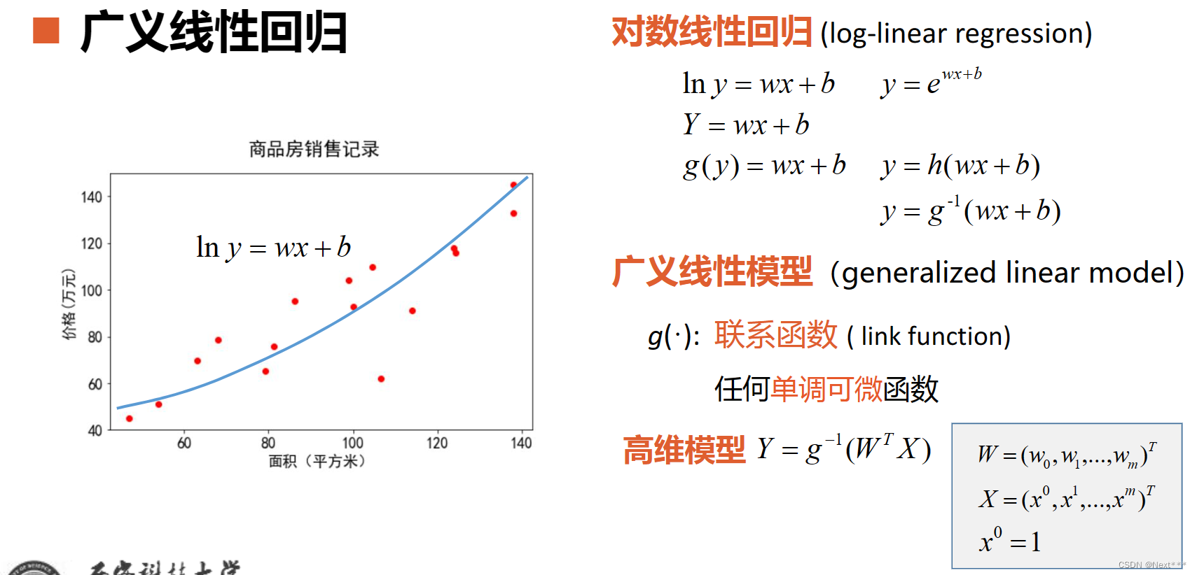
11.1.1 广义线性回归
- 课程回顾
- 线性回归:将自变量和因变量之间的关系,用线性模型来表示;根据已知的样本数据,对未来的、或者未知的数据进行估计
11.1.2 逻辑回归
11.1.2.1 分类问题
- 分类问题:垃圾邮件识别,图片分类,疾病判断
- 分类器:能偶自动对输入的数据进行分类
输入:特征;输出:离散值
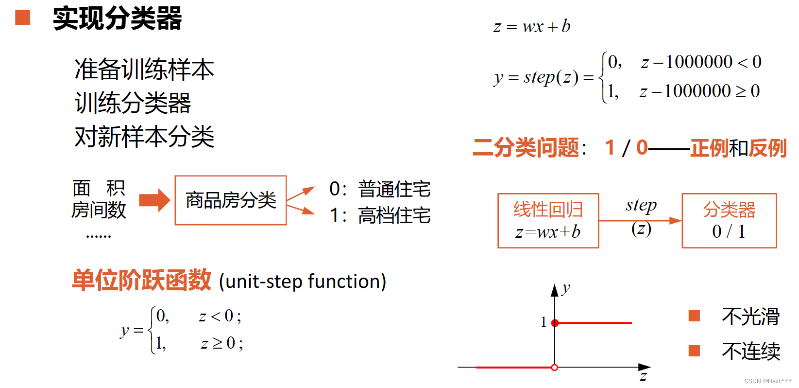
11.1.2.2 实现分类器
-
准备训练样本
-
训练分类器
-
对新样本分类
-
单位阶跃函数(unit-step function)
不光滑
不连续 -
二分类问题 1/0–正例和反例
-
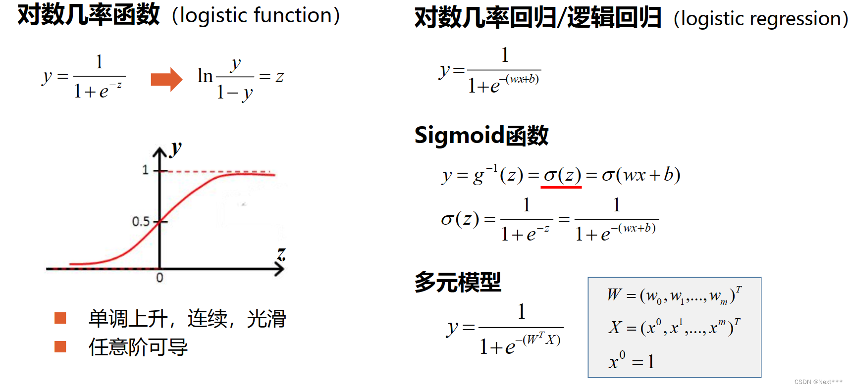
对数几率函数(logistic function):y=1/(1+e−z)y=1/(1+e^{-z})y=1/(1+e−z)
单调上升,连续,光滑
任意阶可导 -
对数几率回归/逻辑回归(logistic regression):y=1/(1+e−(wx+b))y=1/(1+e^{-(wx+b)})y=1/(1+e−(wx+b))
-
Sigmoid函数:形状s的函数,能够将取值范围无穷大的函数转化为一个0到1范围的值;
y=g−1(z)=σ(z)=σ(wx+b)=1/(1+e−z)=1/(1+e−(wx+b))y=g^{-1}(z)=σ(z)=σ(wx+b)=1/(1+e^{-z})=1/(1+e^{-(wx+b)})y=g−1(z)=σ(z)=σ(wx+b)=1/(1+e−z)=1/(1+e−(wx+b)) -
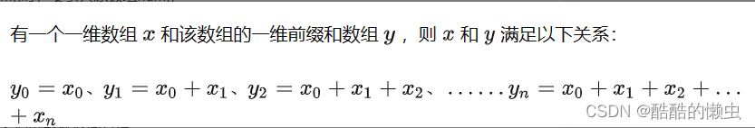
多元模型
y=1/(1+e−(WTX))y = 1/(1+e^{-(W^TX)})y=1/(1+e−(WTX))
W=(w0,w1,…,wm)TW = (w_{0},w_{1},…,w_{m})^{T}W=(w0,w1,…,wm)T
X=(x0,x1,…,xm)TX = (x_{0},x_{1},…,x_{m})^{T}X=(x0,x1,…,xm)T
x0=1x^{0}=1x0=1
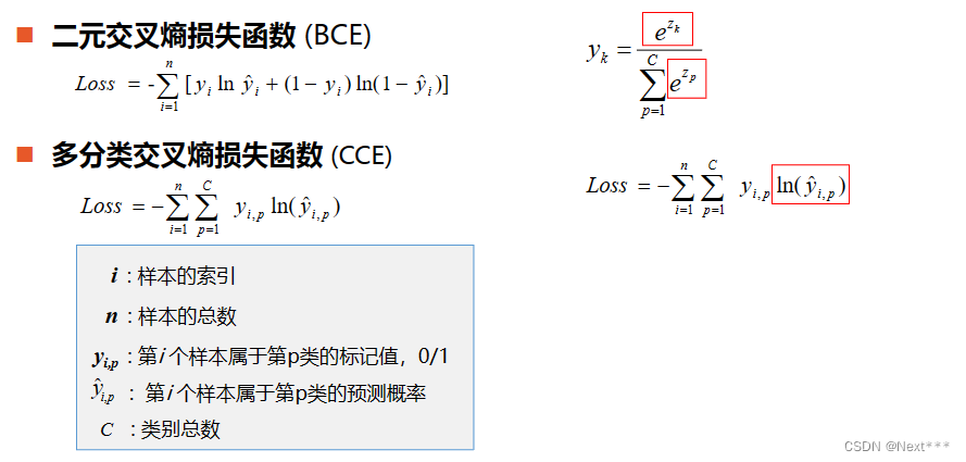
11.1.3 交叉熵损失函数
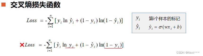
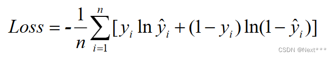
- 交叉熵损失函数
- 每一项误差都是非负的
- 函数值和误差的变化趋势一致
- 凸函数
- 对模型参数求偏导数,无σ’()项
- 平均交叉熵损失函数
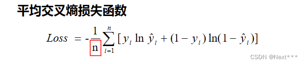
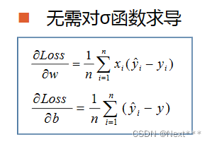
- 偏导数的值只受到标签值和预测值偏差的影响
- 交叉熵损失函数是凸函数,因此使用梯度下降法得到的极小值就是全局最小值
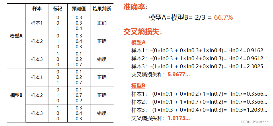
11.1.4 准确率(accuracy)
- 可以使用准确率来评价一个分类器性能
- 准确率=正确分类的样本数/总样本数
- 仅仅通过准确率是无法细分出模型分类器的优劣的
11.1.5 手推三分类问题-交叉熵损失函数,权值更新公式
11.2 实例:实现一元逻辑回归
11.2.1 sigmoid()函数-代码实现
y=1/(1+e−(wx+b))y = 1 / ( 1 + e^{-(wx+b)})y=1/(1+e−(wx+b))
>>> import tensorflow as tf
>>> import numpy as np
>>> x = np.array([1.,2.,3.,4.])
>>> w = tf.Variable(1.)
>>> b = tf.Variable(1.)
>>> y = 1/(1+tf.exp(-(w*x+b)))
>>> y
<tf.Tensor: id=46, shape=(4,), dtype=float32, numpy=array([0.880797  , 0.95257413, 0.98201376, 0.9933072 ], dtype=float32)>
- 注意tf.exp()函数的参数要求是浮点数,否则会报错
11.2.2 交叉熵损失函数-代码实现
>>> import tensorflow as tf
>>> import numpy as np>>> y = np.array([0,0,1,1])
>>> pred=np.array([0.1,0.2,0.8,0.49])>>> # 交叉熵损失函数
>>> -tf.reduce_sum(y*tf.math.log(pred)+(1-y)*tf.math.log(1-pred))
<tf.Tensor: id=58, shape=(), dtype=float64, numpy=1.2649975061637104>>>> # 平均交叉熵巡损失函数
>>> -tf.reduce_mean(y*tf.math.log(pred)+(1-y)*tf.math.log(1-pred))
<tf.Tensor: id=70, shape=(), dtype=float64, numpy=0.3162493765409276>
11.2.3 准确率-代码实现
11.2.3.1 判断阈值是0.5-tf.round()函数
- 准确率=正确分类的样本数/总样本数
>>> import tensorflow as tf
>>> import numpy as np>>> y = np.array([0,0,1,1])
>>> pred=np.array([0.1,0.2,0.8,0.49])>>> # 如果将阈值设为0.5,可以使用四舍五入函数round()将其转换为0或1
>>> tf.round(pred)
<tf.Tensor: id=83, shape=(4,), dtype=float64, numpy=array([0., 0.,
1., 0.])>>>> # 然后使用equal()函数逐元素比较预测值和标签值,得到的结果是一个
和y形状相同的一维张量
>>> tf.equal(tf.round(pred),y)
<tf.Tensor: id=87, shape=(4,), dtype=bool, numpy=array([ True,  True,  True, False])>>>> # 下面使用cast()函数把这个结果转化为整数
>>> tf.cast(tf.equal(tf.round(pred),y),tf.int8)
<tf.Tensor: id=92, shape=(4,), dtype=int8, numpy=array([1, 1, 1, 0], dtype=int8)>>>> # 然后对所有的元素求平均值,就是得到正确样本在所有样本中的比例
>>> tf.reduce_mean(tf.cast(tf.equal(tf.round(pred),y),tf.int8))
<tf.Tensor: id=99, shape=(), dtype=int8, numpy=0>>>> # 记得,如果round()函数,参数是0.5,返回的值是0
>>> tf.round(0.5)
<tf.Tensor: id=101, shape=(), dtype=float32, numpy=0.0>
11.2.3.2 判断阈值不是0.5–where(condition,a,b)函数
where(condition,a,b)
- 根据条件condition返回a或者b的值
- 如果condition中的某个元素为真,对应位置返回a,否则返回b
>>> import tensorflow as tf
>>> import numpy as np>>> y = np.array([0,0,1,1])
>>> pred=np.array([0.1,0.2,0.8,0.49])>>> tf.where(pred<0.5,0,1)
<tf.Tensor: id=105, shape=(4,), dtype=int32, numpy=array([0, 0, 1,
0])>>>> pred<0.5
array([ True,  True, False,  True])>>> tf.where(pred<0.4,0,1)
- 参数a和b还可以是数组或者张量,这时,a和b必须有相同的形状,并且他们的第一维必须和condition形状一致
>>> import tensorflow as tf
>>> import numpy as np>>> pred=np.array([0.1,0.2,0.8,0.49])>>> a = np.array([1,2,3,4])
>>> b = np.array([10,20,30,40])>>> # 当pred中的元素小于0.5时,就返回a中对应位置的元素,否则,返回b中对应位置的元素
>>> tf.where(pred<0.5,a,b)
<tf.Tensor: id=117, shape=(4,), dtype=int32, numpy=array([ 1,  2, 30,  4])>
>>> # 可以看到数组pred中1、2、4个元素都小于0.5,因此取数组a中的元素
,而第3个元素大于0.5,取b中的元素
- 参数a和b也可以省略,这时的返回值数组pred中大于等于0.5的元素的索引,返回值以一个二维张量的形式给出
>>> tf.where(pred>=0.5)
<tf.Tensor: id=119, shape=(1, 1), dtype=int64, numpy=array([[2]], dtype=int64)>
- 下面使用where计算准确率
>>> import tensorflow as tf
>>> import numpy as np
>>> y = np.array([0,0,1,1])
>>> pred=np.array([0.1,0.2,0.8,0.49])  >>> tf.reduce_mean(tf.cast(tf.equal(tf.where(pred<0.5,0,1),y),tf.float32))
<tf.Tensor: id=136, shape=(), dtype=float32, numpy=0.75>
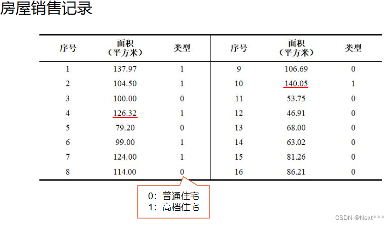
11.2.4 一元逻辑回归-房屋销售记录实例
11.2.4.1 加载数据
# 1 加载数据
import tensorflow as tf
import numpy as np
import matplotlib.pyplot as plt
# 面积
x = np.array([137.97,104.50,100.00,124.32,79.20,99.00,124.00,114.00,106.69,138.05,53.75,46.91,68.00,63.02,81.26,86.21])
# 类型
y = np.array([1,1,0,1,0,1,1,0,0,1,0,0,0,0,0,0])plt.scatter(x,y)
plt.show()
输出结果为:
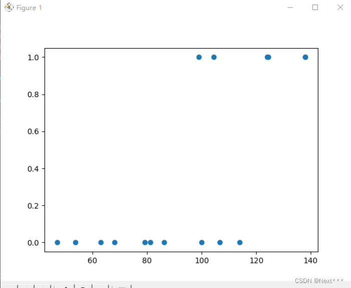
- 类别只有0和1两种
11.2.4.2 数据处理
# 2 数据处理
# sigmoid函数是以0点为中心的,所以对数据中心化
x_train = x - np.mean(x)
y_train = yplt.scatter(x_train,y_train)
plt.show()
输出结果为:
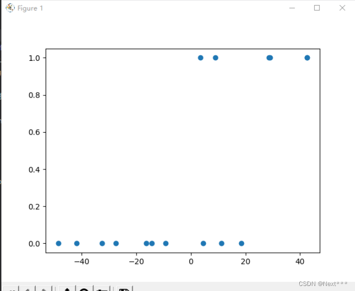
- 可以看到, 这些点整体平移,这些点相对位置不变
11.2.4.3 设置超参数
# 3 设置超参数
learn_rate = 0.005
iter = 5
display_step = 1
11.2.4.4 设置模型变量初始值
# 4 设置模型变量初始值
np.random.seed(612)
w = tf.Variable(np.random.randn())
b = tf.Variable(np.random.randn())
11.2.4.5 训练模型
# 5 训练模型
cross_train = []
acc_train = []for i in range(0,iter+1):with tf.GradientTape() as tape:pred_train = 1/(1+tf.exp(-w*x_train+b))Loss_train = -tf.reduce_mean(y_train*tf.math.log(pred_train)+(1-y_train)*tf.math.log(1-pred_train))Accuracy_train = tf.reduce_mean(tf.cast(tf.equal(tf.where(pred_train<0.5,0,1),y_train),tf.float32))cross_train.append(Loss_train)acc_train.append(Accuracy_train)dL_dw,dL_db = tape.gradient(Loss_train,[w,b])w.assign_sub(learn_rate*dL_dw)b.assign_sub(learn_rate*dL_db)if i % display_step == 0:print("i: %i, Train Loss: %f, Accuracy: %f" % (i,Loss_train,Accuracy_train))
输出结果为:
i: 0, Train Loss: 1.140986, Accuracy: 0.375000
i: 1, Train Loss: 0.703207, Accuracy: 0.625000
i: 2, Train Loss: 0.648479, Accuracy: 0.625000
i: 3, Train Loss: 0.631729, Accuracy: 0.687500
i: 4, Train Loss: 0.624276, Accuracy: 0.687500
i: 5, Train Loss: 0.620331, Accuracy: 0.750000
11.2.4.6 增加sigmoid曲线可视化输出
# 1 加载数据
import tensorflow as tf
import numpy as np
import matplotlib.pyplot as plt
# 面积
x = np.array([137.97,104.50,100.00,124.32,79.20,99.00,124.00,114.00,106.69,138.05,53.75,46.91,68.00,63.02,81.26,86.21])
# 类型
y = np.array([1,1,0,1,0,1,1,0,0,1,0,0,0,0,0,0])# 2 数据处理
# sigmoid函数是以0点为中心的,所以对数据中心化
x_train = x - np.mean(x)
y_train = y# 3 设置超参数
learn_rate = 0.005
iter = 5
display_step = 1# 4 设置模型变量初始值
np.random.seed(612)
w = tf.Variable(np.random.randn())
b = tf.Variable(np.random.randn())x_ = range(-80,80)
y_ = 1/(1+tf.exp(-(w*x_+b)))# 迭代之前,输出数据的散点图
plt.scatter(x_train,y_train)
# 使用初始化参数时的sigmoid曲线
plt.plot(x_,y_,c='r',linewidth=3)# 5 训练模型
cross_train = []
acc_train = []for i in range(0,iter+1):with tf.GradientTape() as tape:pred_train = 1/(1+tf.exp(-w*x_train+b))Loss_train = -tf.reduce_mean(y_train*tf.math.log(pred_train)+(1-y_train)*tf.math.log(1-pred_train))Accuracy_train = tf.reduce_mean(tf.cast(tf.equal(tf.where(pred_train<0.5,0,1),y_train),tf.float32))cross_train.append(Loss_train)acc_train.append(Accuracy_train)dL_dw,dL_db = tape.gradient(Loss_train,[w,b])w.assign_sub(learn_rate*dL_dw)b.assign_sub(learn_rate*dL_db)if i % display_step == 0:print("i: %i, Train Loss: %f, Accuracy: %f" % (i,Loss_train,Accuracy_train))y_ = 1/(1+tf.exp(-(w*x_+b)))plt.plot(x_,y_)# 输出当前权值时的sigmoid曲线
plt.show()
输出结果为:
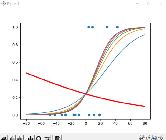
- 红色是使用初始参数时的sigmoid曲线,虽然看起来很离谱,但是恰好属于普通住宅的这10个样本的概率都在0.5以下,所以分类正确率为10/16
- 蓝色是第一次迭代结果
- 紫色是最后一次迭代的结果
- 在0-20之间,出现一段的重合,有一定的交集,所以这个区域中的点可能会出现分类错误,导致准确率无法达到100
- 第一次分类的结果,虽然正确率更大,但是从整体来看,还是经过更多次迭代之后更加合理
11.2.4.7 验证模型
x_test = [128.15,45.00,141.43,106.27,99.00,53.84,85.36,70.00,162.00,114.60]
pred_test = 1/(1+tf.exp(-(w*(x_test-np.mean(x))+b)))
y_test = tf.where(pred_test<0.5,0,1)
for i in range(len(x_test)):print(x_test[i],"\t",pred_test[i].numpy(),"\t",y_test[i].numpy(),"\t")
输出结果为:
128.15   0.84752923      1
45.0     0.003775026     0
141.43   0.94683856      1
106.27   0.4493811       0
99.0     0.30140132      0
53.84    0.008159011     0
85.36    0.11540905      0
70.0     0.032816157     0
162.0    0.99083763      1
114.6    0.62883806      1
11.2.4.8 预测值的sigmoid曲线和散点图
# 1 加载数据
import tensorflow as tf
import numpy as np
import matplotlib.pyplot as plt
# 面积
x = np.array([137.97,104.50,100.00,124.32,79.20,99.00,124.00,114.00,106.69,138.05,53.75,46.91,68.00,63.02,81.26,86.21])
# 类型
y = np.array([1,1,0,1,0,1,1,0,0,1,0,0,0,0,0,0])# 2 数据处理
# sigmoid函数是以0点为中心的,所以对数据中心化
x_train = x - np.mean(x)
y_train = y# 3 设置超参数
learn_rate = 0.005
iter = 5
display_step = 1# 4 设置模型变量初始值
np.random.seed(612)
w = tf.Variable(np.random.randn())
b = tf.Variable(np.random.randn())#x_ = range(-80,80)
#y_ = 1/(1+tf.exp(-(w*x_+b)))# 迭代之前,输出数据的散点图
#plt.scatter(x_train,y_train)
# 使用输出参数时的sigmoid曲线
#plt.plot(x_,y_,c='r',linewidth=3)# 5 训练模型
cross_train = []
acc_train = []for i in range(0,iter+1):with tf.GradientTape() as tape:pred_train = 1/(1+tf.exp(-w*x_train+b))Loss_train = -tf.reduce_mean(y_train*tf.math.log(pred_train)+(1-y_train)*tf.math.log(1-pred_train))Accuracy_train = tf.reduce_mean(tf.cast(tf.equal(tf.where(pred_train<0.5,0,1),y_train),tf.float32))cross_train.append(Loss_train)acc_train.append(Accuracy_train)dL_dw,dL_db = tape.gradient(Loss_train,[w,b])w.assign_sub(learn_rate*dL_dw)b.assign_sub(learn_rate*dL_db)if i % display_step == 0:print("i: %i, Train Loss: %f, Accuracy: %f" % (i,Loss_train,Accuracy_train))#y_ = 1/(1+tf.exp(-(w*x_+b)))#plt.plot(x_,y_)
# 虽然使用x_test表示,但是它们不是测试集,测试集是有标签的数据
x_test = [128.15,45.00,141.43,106.27,99.00,53.84,85.36,70.00,162.00,114.60]
pred_test = 1/(1+tf.exp(-(w*(x_test-np.mean(x))+b)))
y_test = tf.where(pred_test<0.5,0,1)
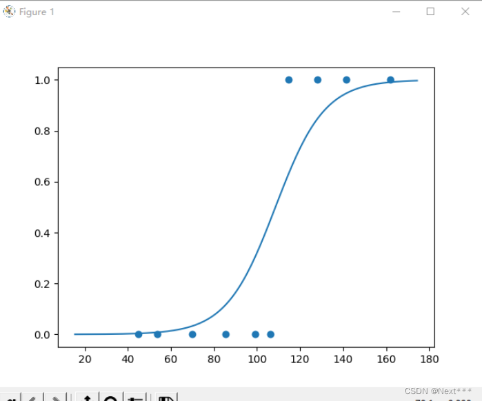
for i in range(len(x_test)):print(x_test[i],"\t",pred_test[i].numpy(),"\t",y_test[i].numpy(),"\t")plt.scatter(x_test,y_test)x_ = range(-80,80)
y_ = 1/(1+tf.exp(-(w*x_+b)))
plt.plot(x_+np.mean(x),y_)plt.show()
输出结果为:
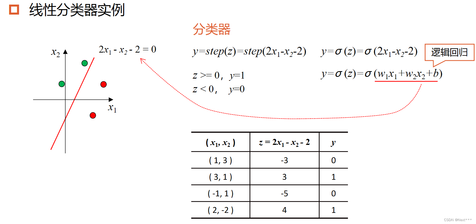
11.3 线性分类器(Linear Classifier)
11.3.1 决策边界-线性可分
- 二维空间中的数据集,如果可以被一条直线分为两类,我们称之为线性可分数据集,这条直线就是一个线性分类器
- 在三维空间中,如果数据集线性可分,是指被一个平面分为两类
- 在一维空间中,所有的点都在一条直线上,线性可分可以理解为可以被一个点分开
- 这里的,分类直线、平面、点被称为决策边界
- 一个m维数据集,
如果可以被一个超平面一分为二,那么这个数据集就是线性可分的,这个超平面就是决策边界
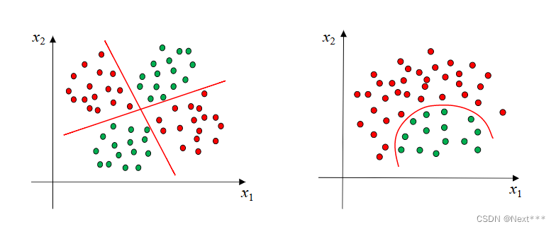
11.3.2 线性不可分
- 线性不可分:样本得两条直线分开,或者一条曲线分开
11.3.3 逻辑运算
11.3.3.1 线性可分-与、或、非
-
在逻辑运算中,与&、或|、非!都是线性可分的
-
显然可以通过训练得到对应的分类器,并且一定收敛
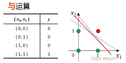
-
与运算
-
或运算
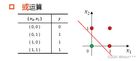
-
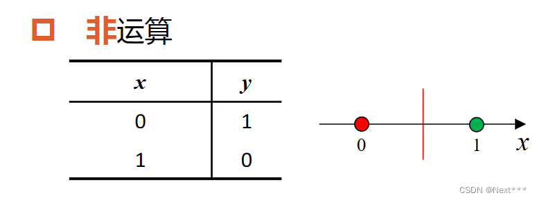
非运算
11.3.3.2 线性不可分-异或
- 异或运算,也可以看作是按类加运算
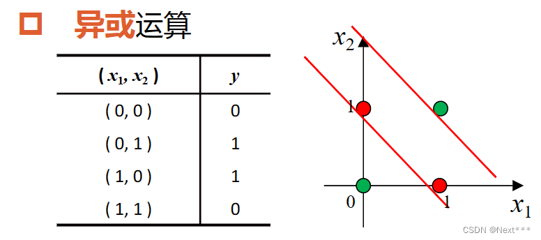
- 显然,要分开它,最少得两条直线
11.4 实例:实现多元逻辑回归
11.4.1 实现多元逻辑回归
11.4.1.1 鸢尾花数据集(iris)再次介绍
- 在这里,使用逻辑回归实现对鸢尾花(iris)的分类
- Iris数据集
- 150个样本
- 4个属性:花萼长度(Sepal Length)、花萼宽度(Sepal Width)、花瓣长度(Petal Length)、花瓣宽度(Petal Width)
- 1个标签:山鸢尾(Setosa)、变色鸢尾(Versicolour)、维吉尼亚鸢尾(Virginica)
- 属性两两可视化后的结果为:
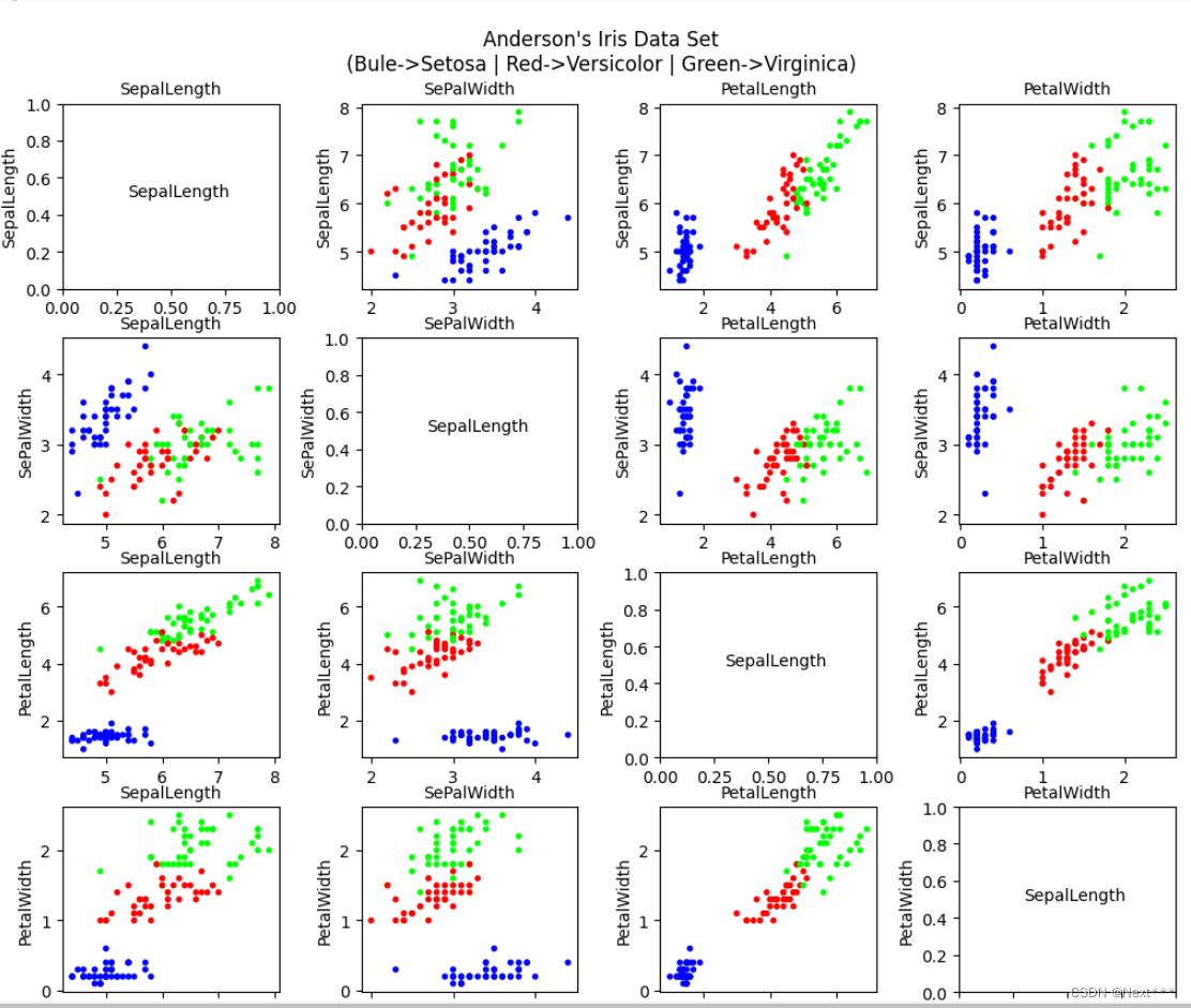
山鸢尾(蓝色)、变色鸢尾(红色)、维吉尼亚鸢尾(绿色)
-
蓝色的与其他两个差别大,选择任何两个都可以区分开;所以选择蓝色(山鸢尾)的和红色(变色鸢尾)两种鸢尾花,花萼长度和花萼宽度两种属性,通过逻辑回归实现对他们的分类
-
了解鸢尾花数据集的具体使用方法可以参考Lesson6—Matplotlib数据可视化中的6.5节
11.4.1.2 实现多元逻辑回归
11.4.1.2.1 加载数据
# 1 加载数据
import tensorflow as tf
import pandas as pd
import numpy as np
import matplotlib as mpl
import matplotlib.pyplot as pltTRAIN_URL = "http://download.tensorflow.org/data/iris_training.csv"
train_path = tf.keras.utils.get_file(TRAIN_URL.split('/')[-1],TRAIN_URL)df_iris = pd.read_csv(train_path,header=0) # 是一个pandas二维数据表
11.4.1.2.2 处理数据
11.4.1.2.2.1 自己定义色彩方案mpl.colors.ListedColormap()
11.4.1.2.2.2 无须归一化,只需中心化
# 2 处理数据
# 首先将二维数据表转化为numpy数组
iris= np.array(df_iris)  # shape(120,5)# 提取属性和标签
train_x = iris[:,0:2]  # (120,2)
train_y = iris[:,4] # (120,)# 提取山鸢尾和变色鸢尾,提取出标签纸为0和1的值
x_train = train_x[train_y < 2] # (78,2)
y_train = train_y[train_y < 2] # (78,)# 记录现在的样本数
num = len(x_train)
# 中心化处理
x_train = x_train - np.mean(x_train,axis= 0)# 生成多元模型的属性矩阵和标签列向量
x0_train = np.ones(num).reshape(-1,1)
X = tf.cast(tf.concat((x0_train,x_train),axis=1),tf.float32) # shape(78,3)
Y = tf.cast(y_train.reshape(-1,1),tf.float32) # shape(78,1)
# 可视化样本
#cm_pt = mpl.colors.ListedColormap(["blue","red"]) # 设置色彩方案
#plt.scatter(x_train[:,0],x_train[:,1],c=y_train,cmap=cm_pt)
#plt.show()
处理结果为:

- 可以看到中心化之后,样本点被平移,样本点的横坐标和纵坐标都是0
11.4.1.2.3 设置超参数
# 3 设置超参数
learn_rate = 0.2
iter = 120
display_step = 30
11.4.1.2.4 设置模型参数初始值
# 4 设置模型参数初始值
np.random.seed(612)
W = tf.Variable(np.random.randn(3,1),dtype=tf.float32)
11.4.1.2.5 训练模型
# 5 训练模型
ce = []
acc = []for i in range(0,iter+1):with tf.GradientTape() as tape:PRED = 1/(1+tf.exp(-tf.matmul(X,W))) # 每个样本的预测概率Loss = -tf.reduce_mean(Y*tf.math.log(PRED)+(1-Y)*tf.math.log(1-PRED))accuracy = tf.reduce_mean(tf.cast(tf.equal(tf.where(PRED.numpy()<0.5,0.,1.),Y),tf.float32))ce.append(Loss)acc.append(accuracy)dL_dW = tape.gradient(Loss,W)W.assign_sub(learn_rate*dL_dW)if i % display_step ==0:print("i: %i, Acc: %f, Loss: %f" % (i,accuracy,Loss))
输出结果为:
i: 0, Acc: 0.230769, Loss: 0.994269
i: 30, Acc: 0.961538, Loss: 0.481892
i: 60, Acc: 0.987179, Loss: 0.319128
i: 90, Acc: 0.987179, Loss: 0.246626
i: 120, Acc: 1.000000, Loss: 0.204982
11.4.1.2.6 代码汇总(包含前五个步骤)
# 1 加载数据
import tensorflow as tf
import pandas as pd
import numpy as np
import matplotlib as mpl
import matplotlib.pyplot as pltTRAIN_URL = "http://download.tensorflow.org/data/iris_training.csv"
train_path = tf.keras.utils.get_file(TRAIN_URL.split('/')[-1],TRAIN_URL)df_iris = pd.read_csv(train_path,header=0) # 是一个pandas二维数据表# 2 处理数据
# 首先将二维数据表转化为numpy数组
iris= np.array(df_iris)  # shape(120,5)# 提取属性和标签
train_x = iris[:,0:2]  # (120,2)
train_y = iris[:,4] # (120,)# 提取山鸢尾和变色鸢尾,提取出标签纸为0和1的值
x_train = train_x[train_y < 2] # (78,2)
y_train = train_y[train_y < 2] # (78,)# 记录现在的样本数
num = len(x_train)
# 中心化处理
x_train = x_train - np.mean(x_train,axis= 0)# 生成多元模型的属性矩阵和标签列向量
x0_train = np.ones(num).reshape(-1,1)
X = tf.cast(tf.concat((x0_train,x_train),axis=1),tf.float32) # shape(78,3)
Y = tf.cast(y_train.reshape(-1,1),tf.float32) # shape(78,1)
# 可视化样本
#cm_pt = mpl.colors.ListedColormap(["blue","red"]) # 设置色彩方案
#plt.scatter(x_train[:,0],x_train[:,1],c=y_train,cmap=cm_pt)
#plt.show()# 3 设置超参数
learn_rate = 0.2
iter = 120
display_step = 30# 4 设置模型参数初始值
np.random.seed(612)
W = tf.Variable(np.random.randn(3,1),dtype=tf.float32)# 5 训练模型
ce = []
acc = []for i in range(0,iter+1):with tf.GradientTape() as tape:PRED = 1/(1+tf.exp(-tf.matmul(X,W))) # 每个样本的预测概率Loss = -tf.reduce_mean(Y*tf.math.log(PRED)+(1-Y)*tf.math.log(1-PRED))accuracy = tf.reduce_mean(tf.cast(tf.equal(tf.where(PRED.numpy()<0.5,0.,1.),Y),tf.float32))ce.append(Loss)acc.append(accuracy)dL_dW = tape.gradient(Loss,W)W.assign_sub(learn_rate*dL_dW)if i % display_step ==0:print("i: %i, Acc: %f, Loss: %f" % (i,accuracy,Loss))
11.4.1.2.6 可视化
11.4.1.2.6.1 绘制损失和准确率变化曲线
# 损失和准确率变化曲线
plt.figure(figsize=(5,3))
plt.plot(ce,c='b',label="Loss")
plt.plot(acc,c='r',label="acc")
plt.legend()
plt.show()
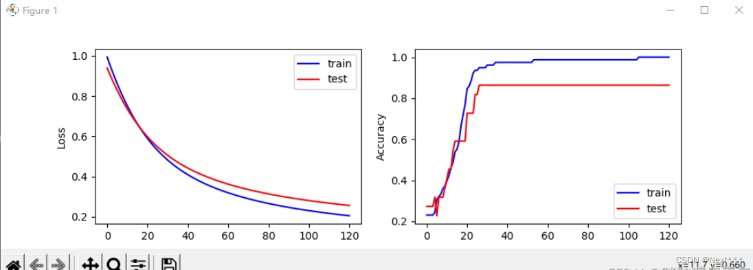
输出结果为:
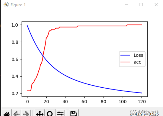
- 损失一直单调下降,所以损失下降曲线很光滑
- 而准确率上升到一定的数值之后,有时候会停留在某个时间一段时间,因此呈现出台阶上升的趋势
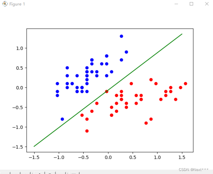
11.4.1.2.6.2 绘制决策边界
# 绘制决策边界
cm_pt = mpl.colors.ListedColormap(["blue","red"]) # 设置色彩方案
plt.scatter(x_train[:,0],x_train[:,1],c=y_train,cmap=cm_pt)
x_ = [-1.5,1.5]
y_ = -(W[1]*x_+W[0])/W[2]
plt.plot(x_,y_,c='g')
plt.show()
输出结果为:
11.4.1.2.6.3 在训练过程中绘制决策边界
# 1 加载数据
import tensorflow as tf
import pandas as pd
import numpy as np
import matplotlib as mpl
import matplotlib.pyplot as pltTRAIN_URL = "http://download.tensorflow.org/data/iris_training.csv"
train_path = tf.keras.utils.get_file(TRAIN_URL.split('/')[-1],TRAIN_URL)df_iris = pd.read_csv(train_path,header=0) # 是一个pandas二维数据表# 2 处理数据
# 首先将二维数据表转化为numpy数组
iris= np.array(df_iris)  # shape(120,5)# 提取属性和标签
train_x = iris[:,0:2]  # (120,2)
train_y = iris[:,4] # (120,)# 提取山鸢尾和变色鸢尾,提取出标签纸为0和1的值
x_train = train_x[train_y < 2] # (78,2)
y_train = train_y[train_y < 2] # (78,)# 记录现在的样本数
num = len(x_train)
# 中心化处理
x_train = x_train - np.mean(x_train,axis= 0)# 生成多元模型的属性矩阵和标签列向量
x0_train = np.ones(num).reshape(-1,1)
X = tf.cast(tf.concat((x0_train,x_train),axis=1),tf.float32) # shape(78,3)
Y = tf.cast(y_train.reshape(-1,1),tf.float32) # shape(78,1)
# 可视化样本
#cm_pt = mpl.colors.ListedColormap(["blue","red"]) # 设置色彩方案
#plt.scatter(x_train[:,0],x_train[:,1],c=y_train,cmap=cm_pt)
#plt.show()# 3 设置超参数
learn_rate = 0.2
iter = 120
display_step = 30# 4 设置模型参数初始值
np.random.seed(612)
W = tf.Variable(np.random.randn(3,1),dtype=tf.float32)cm_pt = mpl.colors.ListedColormap(["blue","red"]) # 设置色彩方案x_ = [-1.5,1.5]
y_ = -(W[0]+W[1]*x_)/W[2]plt.scatter(x_train[:,0],x_train[:,1],c=y_train,cmap=cm_pt)
plt.plot(x_,y_,c='r',linewidth=3)
plt.xlim([-1.5,1.5])
plt.ylim([-1.5,1.5])# 5 训练模型
ce = []
acc = []for i in range(0,iter+1):with tf.GradientTape() as tape:PRED = 1/(1+tf.exp(-tf.matmul(X,W))) # 每个样本的预测概率Loss = -tf.reduce_mean(Y*tf.math.log(PRED)+(1-Y)*tf.math.log(1-PRED))accuracy = tf.reduce_mean(tf.cast(tf.equal(tf.where(PRED.numpy()<0.5,0.,1.),Y),tf.float32))ce.append(Loss)acc.append(accuracy)dL_dW = tape.gradient(Loss,W)W.assign_sub(learn_rate*dL_dW)if i % display_step ==0:print("i: %i, Acc: %f, Loss: %f" % (i,accuracy,Loss))y_ = -(W[0]+W[1]*x_)/W[2]plt.plot(x_,y_)plt.show()
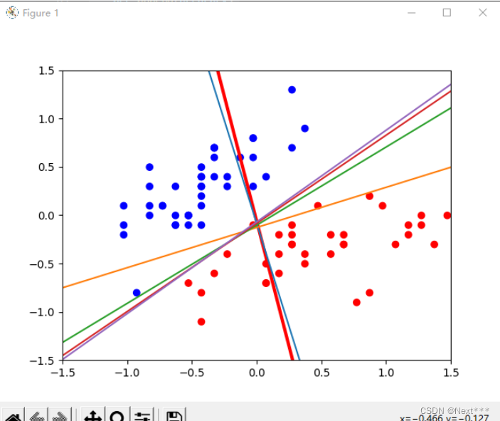
- 红色的是初始的,之后慢慢调增
11.4.1.2.7 使用测试集
# 1 加载数据
import tensorflow as tf
import pandas as pd
import numpy as np
import matplotlib as mpl
import matplotlib.pyplot as pltTRAIN_URL = "http://download.tensorflow.org/data/iris_training.csv"
TEST_URL = "http://download.tensorflow.org/data/iris_test.csv"
train_path = tf.keras.utils.get_file(TRAIN_URL.split('/')[-1],TRAIN_URL)
test_path = tf.keras.utils.get_file(TEST_URL.split('/')[-1],TEST_URL)df_iris_train = pd.read_csv(train_path,header=0) # 是一个pandas二维数据表
df_iris_test =  pd.read_csv(test_path,header=0)# 2 处理数据
# 首先将二维数据表转化为numpy数组
iris_train= np.array(df_iris_train)  # shape(120,5)
iris_test= np.array(df_iris_test)  # shape(30,5)# 提取属性和标签
train_x = iris_train[:,0:2]  # (120,2)
train_y = iris_train[:,4] # (120,)test_x = iris_test[:,0:2]  # (30,2)
test_y = iris_test[:,4] # (30,)
# 提取山鸢尾和变色鸢尾,提取出标签纸为0和1的值
x_train = train_x[train_y < 2] # (78,2)
y_train = train_y[train_y < 2] # (78,)x_test = test_x[test_y < 2] # (22,2)
y_test = test_y[test_y < 2] # (22,)
# 记录现在的样本数
num_train = len(x_train)
num_test = len(x_test)
# 分别进行按列中心化处理,要求训练集和测试集独立同分布的,具有相同的均值和方差,数量有限的情况下,只要尽量接近即可
# 使用划分好的不用太考虑,但是自己划分数据集,要考虑这点
x_train = x_train - np.mean(x_train,axis= 0)
x_test = x_test - np.mean(x_test,axis=0)# 生成多元模型的属性矩阵和标签列向量
x0_train = np.ones(num_train).reshape(-1,1)
X_train = tf.cast(tf.concat((x0_train,x_train),axis=1),tf.float32) # shape(78,3)
Y_train = tf.cast(y_train.reshape(-1,1),tf.float32) # shape(78,1)x0_test = np.ones(num_test).reshape(-1,1)
X_test = tf.cast(tf.concat((x0_test,x_test),axis=1),dtype=tf.float32) # (22,3)
Y_test = tf.cast(y_test.reshape(-1,1),dtype=tf.float32) # (22,1)# 可视化样本
#cm_pt = mpl.colors.ListedColormap(["blue","red"]) # 设置色彩方案
#plt.scatter(x_train[:,0],x_train[:,1],c=y_train,cmap=cm_pt)
#plt.show()# 3 设置超参数
learn_rate = 0.2
iter = 120
display_step = 30# 4 设置模型参数初始值
np.random.seed(612)
W = tf.Variable(np.random.randn(3,1),dtype=tf.float32)cm_pt = mpl.colors.ListedColormap(["blue","red"]) # 设置色彩方案x_ = [-1.5,1.5]
y_ = -(W[0]+W[1]*x_)/W[2]# 5 训练模型
ce_train = []
acc_train = []
ce_test = []
acc_test = []for i in range(0,iter+1):with tf.GradientTape() as tape:PRED_train = 1/(1+tf.exp(-tf.matmul(X_train,W))) # 每个样本的预测概率Loss_train = -tf.reduce_mean(Y_train*tf.math.log(PRED_train)+(1-Y_train)*tf.math.log(1-PRED_train))PRED_test = 1/(1+tf.exp(-tf.matmul(X_test,W))) # 每个样本的预测概率Loss_test = -tf.reduce_mean(Y_test*tf.math.log(PRED_test)+(1-Y_test)*tf.math.log(1-PRED_test))accuracy_train = tf.reduce_mean(tf.cast(tf.equal(tf.where(PRED_train.numpy()<0.5,0.,1.),Y_train),tf.float32))accuracy_test = tf.reduce_mean(tf.cast(tf.equal(tf.where(PRED_test.numpy()<0.5,0.,1.),Y_test),tf.float32))ce_train.append(Loss_train)acc_train.append(accuracy_train)ce_test.append(Loss_test)acc_test.append(accuracy_test)dL_dW = tape.gradient(Loss_train,W)W.assign_sub(learn_rate*dL_dW)if i % display_step ==0:print("i: %i, TrainAcc: %f, TrainLoss: %f, TestAcc: %f, TestLoss: %f" % (i,accuracy_train,Loss_train,accuracy_test,Loss_test))# 6 可视化
plt.figure(figsize=(10,3))plt.subplot(121)
plt.plot(ce_train,c='b',label="train")
plt.plot(ce_test,c='r',label="test")
plt.ylabel("Loss")
plt.legend()plt.subplot(122)
plt.plot(acc_train,c='b',label="train")
plt.plot(acc_test,c='r',label="test")
plt.ylabel("Accuracy")plt.legend()
plt.show()
输出结果为:
i: 0, TrainAcc: 0.230769, TrainLoss: 0.994269, TestAcc: 0.272727, TestLoss: 0.939684
i: 30, TrainAcc: 0.961538, TrainLoss: 0.481892, TestAcc: 0.863636, TestLoss: 0.505456
i: 60, TrainAcc: 0.987179, TrainLoss: 0.319128, TestAcc: 0.863636, TestLoss: 0.362112
i: 90, TrainAcc: 0.987179, TrainLoss: 0.246626, TestAcc: 0.863636, TestLoss: 0.295611
i: 120, TrainAcc: 1.000000, TrainLoss: 0.204982, TestAcc: 0.863636, TestLoss: 0.256212
11.4.2 绘制分类图
11.4.2.1 生成网格坐标矩阵np.meshgrid()
X,Y = np.meshgrid(x,y)
11.4.2.2 填充网格 plt.pcolomesh()
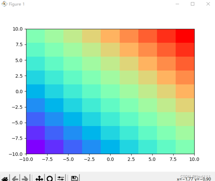
11.4.2.2.1 rainbow色彩方案
plt.pcolomesh(X,Y,Z,cmap)
- 前两个参数:X和Y确定网格位置
- 第三个参数:Z决定网格的颜色
- 第四个参数:cmap指定所使用的颜色方案
- 可以使用plt.contourf()函数代替plt.pcolomesh()函数
# 1 加载数据
import tensorflow as tf
import numpy as np
import matplotlib as mpl
import matplotlib.pyplot as pltn = 10
x = np.linspace(-10,10,n)
y = np.linspace(-10,10,n)
X,Y = np.meshgrid(x,y)
Z = X+Y
plt.pcolormesh(X,Y,Z,cmap="rainbow")plt.show()
输出结果为:
11.4.2.2.2 自己定义的色彩方案
- 如果定义了两种颜色,就平均按照颜色值划分两类,如果是三种颜色,就划分为三个区域
# 1 加载数据
import tensorflow as tf
import numpy as np
import matplotlib as mpl
import matplotlib.pyplot as pltn = 200
x = np.linspace(-10,10,n)
y = np.linspace(-10,10,n)
X,Y = np.meshgrid(x,y)
Z = X+Y
cm_bg = mpl.colors.ListedColormap(["#FFA0A0","#A0FFA0"])
plt.pcolormesh(X,Y,Z,cmap=cm_bg)plt.show()
输出结果为:

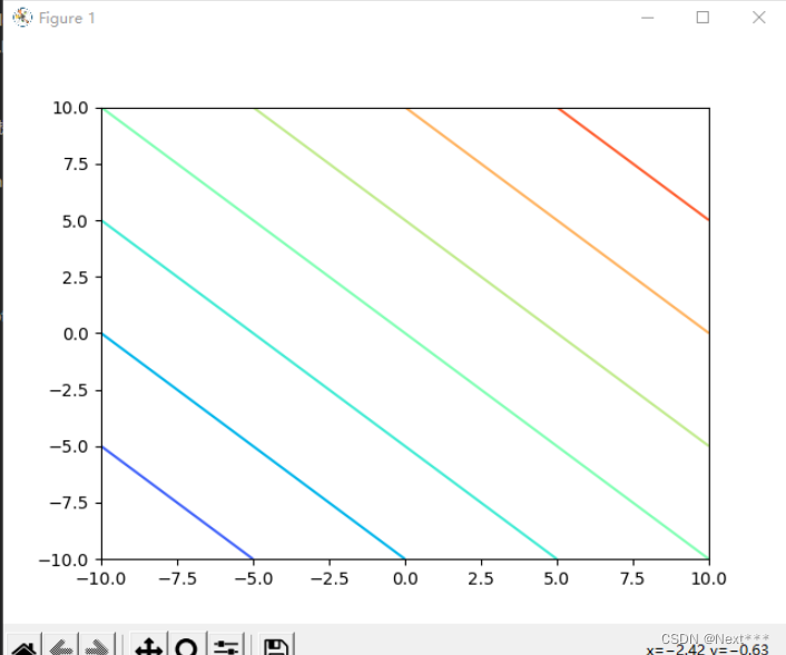
11.4.2.3 绘制轮廓线plt.contour()
- plt.contour():根据类的取值绘制出相同取值的边界
- 可以理解为三维模型的等高线
# 1 加载数据
import tensorflow as tf
import numpy as np
import matplotlib as mpl
import matplotlib.pyplot as pltn = 200
x = np.linspace(-10,10,n)
y = np.linspace(-10,10,n)
X,Y = np.meshgrid(x,y)
Z = X+Yplt.contour(X,Y,Z,cmap="rainbow")plt.show()
输出结果为:
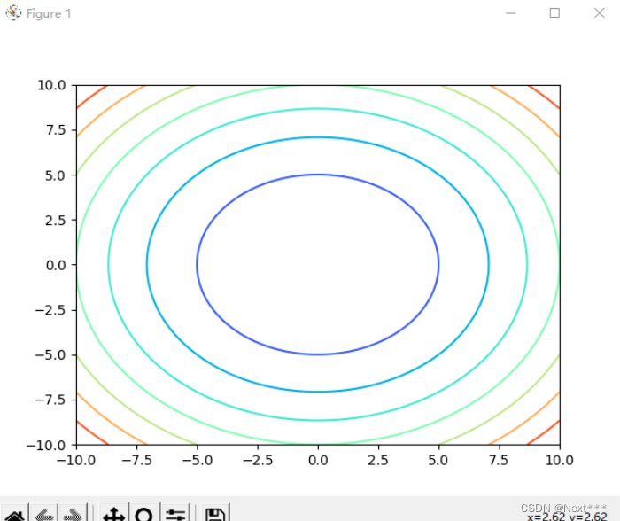
修改为
Z = X**2+Y**2
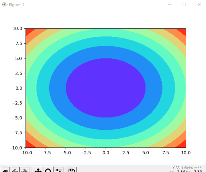
11.4.2.3.1 给轮廓线之间填充颜色plt.contourf(X,Y,Z,a,cmap)
- 填充分区
plt.contourf(X,Y,Z,a,cmap)
-
前两个参数:X和Y确定网格位置
-
第三个参数:Z决定网格的颜色
-
第四个参数:a,指定颜色细分的数量
-
第五个参数:cmap指定所使用的颜色方案
-
可以使用plt.contourf()函数代替plt.pcolomesh()函数
# 1 加载数据
import tensorflow as tf
import numpy as np
import matplotlib as mpl
import matplotlib.pyplot as pltn = 200
x = np.linspace(-10,10,n)
y = np.linspace(-10,10,n)
X,Y = np.meshgrid(x,y)
Z = X**2+Y**2plt.contourf(X,Y,Z,cmap="rainbow")plt.show()
输出结果为:
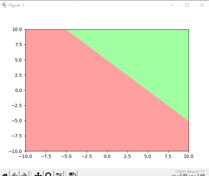
11.4.2.4 绘制分类图例子
# 1 加载数据
import tensorflow as tf
import numpy as np
import matplotlib as mpl
import matplotlib.pyplot as pltn = 200
x = np.linspace(-10,10,n)
y = np.linspace(-10,10,n)
X,Y = np.meshgrid(x,y)
Z = X+Ycm_bg = mpl.colors.ListedColormap(["#FFA0A0","#A0FFA0"])
Z = tf.where(Z<5,0,1)
plt.contourf(X,Y,Z,cmap=cm_bg)plt.show()
输出结果为:
11.4.2.5 根据鸢尾花分类模型,绘制训练集和测试集分类图
# 1 加载数据
import tensorflow as tf
import pandas as pd
import numpy as np
import matplotlib as mpl
import matplotlib.pyplot as pltTRAIN_URL = "http://download.tensorflow.org/data/iris_training.csv"
TEST_URL = "http://download.tensorflow.org/data/iris_test.csv"
train_path = tf.keras.utils.get_file(TRAIN_URL.split('/')[-1],TRAIN_URL)
test_path = tf.keras.utils.get_file(TEST_URL.split('/')[-1],TEST_URL)df_iris_train = pd.read_csv(train_path,header=0) # 是一个pandas二维数据表
df_iris_test = pd.read_csv(test_path,header=0)# 2 处理数据
# 首先将二维数据表转化为numpy数组
iris_train= np.array(df_iris_train) # shape(120,5)
iris_test= np.array(df_iris_test) # shape(30,5)# 提取属性和标签
train_x = iris_train[:,0:2] # (120,2)
train_y = iris_train[:,4] # (120,)test_x = iris_test[:,0:2] # (30,2)
test_y = iris_test[:,4] # (30,)
# 提取山鸢尾和变色鸢尾,提取出标签纸为0和1的值
x_train = train_x[train_y < 2] # (78,2)
y_train = train_y[train_y < 2] # (78,)x_test = test_x[test_y < 2] # (22,2)
y_test = test_y[test_y < 2] # (22,)
# 记录现在的样本数
num_train = len(x_train)
num_test = len(x_test)
# 分别进行按列中心化处理,要求训练集和测试集独立同分布的,具有相同的均值和方差,数量有限的情况下,只要尽量接近即可
# 使用划分好的不用太考虑,但是自己划分数据集,要考虑这点
x_train = x_train - np.mean(x_train,axis= 0)
x_test = x_test - np.mean(x_test,axis=0)# 生成多元模型的属性矩阵和标签列向量
x0_train = np.ones(num_train).reshape(-1,1)
X_train = tf.cast(tf.concat((x0_train,x_train),axis=1),tf.float32) # shape(78,3)
Y_train = tf.cast(y_train.reshape(-1,1),tf.float32) # shape(78,1)x0_test = np.ones(num_test).reshape(-1,1)
X_test = tf.cast(tf.concat((x0_test,x_test),axis=1),dtype=tf.float32) # (22,3)
Y_test = tf.cast(y_test.reshape(-1,1),dtype=tf.float32) # (22,1)# 可视化样本
#cm_pt = mpl.colors.ListedColormap(["blue","red"]) # 设置色彩方案
#plt.scatter(x_train[:,0],x_train[:,1],c=y_train,cmap=cm_pt)
#plt.show()# 3 设置超参数
learn_rate = 0.2
iter = 120
display_step = 30# 4 设置模型参数初始值
np.random.seed(612)
W = tf.Variable(np.random.randn(3,1),dtype=tf.float32)cm_pt = mpl.colors.ListedColormap(["blue","red"]) # 设置色彩方案x_ = [-1.5,1.5]
y_ = -(W[0]+W[1]*x_)/W[2]# 5 训练模型
ce_train = []
acc_train = []
ce_test = []
acc_test = []for i in range(0,iter+1):with tf.GradientTape() as tape:PRED_train = 1/(1+tf.exp(-tf.matmul(X_train,W))) # 每个样本的预测概率Loss_train = -tf.reduce_mean(Y_train*tf.math.log(PRED_train)+(1-Y_train)*tf.math.log(1-PRED_train))PRED_test = 1/(1+tf.exp(-tf.matmul(X_test,W))) # 每个样本的预测概率Loss_test = -tf.reduce_mean(Y_test*tf.math.log(PRED_test)+(1-Y_test)*tf.math.log(1-PRED_test))accuracy_train = tf.reduce_mean(tf.cast(tf.equal(tf.where(PRED_train.numpy()<0.5,0.,1.),Y_train),tf.float32))accuracy_test = tf.reduce_mean(tf.cast(tf.equal(tf.where(PRED_test.numpy()<0.5,0.,1.),Y_test),tf.float32))ce_train.append(Loss_train)acc_train.append(accuracy_train)ce_test.append(Loss_test)acc_test.append(accuracy_test)dL_dW = tape.gradient(Loss_train,W)W.assign_sub(learn_rate*dL_dW)if i % display_step ==0:print("i: %i, TrainAcc: %f, TrainLoss: %f, TestAcc: %f, TestLoss: %f" % (i,accuracy_train,Loss_train,accuracy_test,Loss_test))# 6 可视化
# 根据鸢尾花分类模型,绘制分类图
# 定义绘制散点的颜色方案
cm_pt = mpl.colors.ListedColormap(["blue","red"])
# 定义背景颜色方案
cm_bg = mpl.colors.ListedColormap(["#FFA0A0","#A0FFA0"])
plt.rcParams['font.sans-serif']="SimHei"plt.figure(figsize=(15,5))# 绘制训练集
plt.subplot(121)
M = 300
x1_min,x2_min = x_train.min(axis=0)
x1_max,x2_max = x_train.max(axis=0)
t1 = np.linspace(x1_min,x1_max,M) # 使用花萼长度的取值范围作为横坐标取值范围
t2 = np.linspace(x2_min,x2_max,M) # 使用花萼宽度的取值范围作为纵坐标取值范围
m1,m2 = np.meshgrid(t1,t2) # 生成网格点坐标矩阵m0 = np.ones(M*M)
# 生成多元线性模型需要的属性矩阵
X_mesh = tf.cast(np.stack((m0,m1.reshape(-1),m2.reshape(-1)),axis=1),dtype=tf.float32)
# 使用训练得到的W,根据sigmoid公式计算所有网格点对应的函数值
Y_mesh = tf.cast(1/(1+tf.exp(-tf.matmul(X_mesh,W))),dtype=tf.float32)
# 把分类结果转化为0,1,作为填充粉色,还是绿色的依据
Y_mesh = tf.where(Y_mesh<0.5,0,1)# 并对其进行唯独变换,使其和m1,m2有相同的形状
n = tf.reshape(Y_mesh,m1.shape)# 注意,TensorFlow中的绘图是有层次的,首先绘制分区图作为背景,然后在上面绘制散点图
# 绘制分区图
plt.pcolormesh(m1,m2,n,cmap=cm_bg)
# 绘制散点图
plt.scatter(x_train[:,0],x_train[:,1],c=y_train,cmap=cm_pt)
plt.title("训练集分类图",fontsize = 14)
plt.legend()# 绘制测试集
plt.subplot(122)
M = 300
x1_min,x2_min = x_test.min(axis=0)
x1_max,x2_max = x_test.max(axis=0)
t1 = np.linspace(x1_min,x1_max,M) # 使用花萼长度的取值范围作为横坐标取值范围
t2 = np.linspace(x2_min,x2_max,M) # 使用花萼宽度的取值范围作为纵坐标取值范围
m1,m2 = np.meshgrid(t1,t2) # 生成网格点坐标矩阵m0 = np.ones(M*M)
# 生成多元线性模型需要的属性矩阵
X_mesh = tf.cast(np.stack((m0,m1.reshape(-1),m2.reshape(-1)),axis=1),dtype=tf.float32)
# 使用训练得到的W,根据sigmoid公式计算所有网格点对应的函数值
Y_mesh = tf.cast(1/(1+tf.exp(-tf.matmul(X_mesh,W))),dtype=tf.float32)
# 把分类结果转化为0,1,作为填充粉色,还是绿色的依据
Y_mesh = tf.where(Y_mesh<0.5,0,1)# 并对其进行唯独变换,使其和m1,m2有相同的形状
n = tf.reshape(Y_mesh,m1.shape)# 注意,TensorFlow中的绘图是有层次的,首先绘制分区图作为背景,然后在上面绘制散点图
# 绘制分区图
plt.pcolormesh(m1,m2,n,cmap=cm_bg)
# 绘制散点图
plt.scatter(x_test[:,0],x_test[:,1],c=y_test,cmap=cm_pt)
plt.title("测试集分类图",fontsize = 14)
plt.legend()plt.show()
x1_max,x2_max = x_train.max(axis=0)
t1 = np.linspace(x1_min,x1_max,M) # 使用花萼长度的取值范围作为横坐标取值范围
t2 = np.linspace(x2_min,x2_max,M) # 使用花萼宽度的取值范围作为纵坐标取值范围
m1,m2 = np.me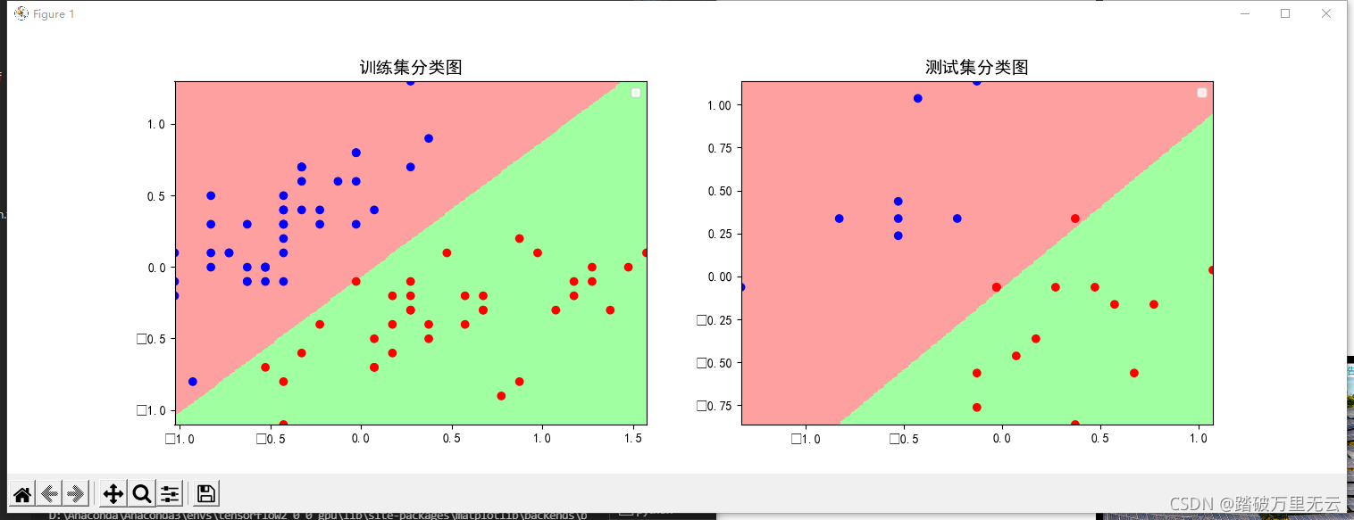
shgrid(t1,t2) # 生成网格点坐标矩阵m0 = np.ones(M*M)
# 生成多元线性模型需要的属性矩阵
X_mesh = tf.cast(np.stack((m0,m1.reshape(-1),m2.reshape(-1)),axis=1),dtype=tf.float32)
# 使用训练得到的W,根据sigmoid公式计算所有网格点对应的函数值
Y_mesh = tf.cast(1/(1+tf.exp(-tf.matmul(X_mesh,W))),dtype=tf.float32)
# 把分类结果转化为0,1,作为填充粉色,还是绿色的依据
Y_mesh = tf.where(Y_mesh<0.5,0,1)# 并对其进行唯独变换,使其和m1,m2有相同的形状
n = tf.reshape(Y_mesh,m1.shape)# 注意,TensorFlow中的绘图是有层次的,首先绘制分区图作为背景,然后在上面绘制散点图
# 绘制分区图
plt.pcolormesh(m1,m2,n,cmap=cm_bg)
# 绘制散点图
plt.scatter(x_train[:,0],x_train[:,1],c=y_train,cmap=cm_pt)# 绘制测试集
plt.subplot(122)
M = 300
x1_min,x2_min = x_test.min(axis=0)
x1_max,x2_max = x_test.max(axis=0)
t1 = np.linspace(x1_min,x1_max,M) # 使用花萼长度的取值范围作为横坐标取值范围
t2 = np.linspace(x2_min,x2_max,M) # 使用花萼宽度的取值范围作为纵坐标取值范围
m1,m2 = np.meshgrid(t1,t2) # 生成网格点坐标矩阵m0 = np.ones(M*M)
# 生成多元线性模型需要的属性矩阵
X_mesh = tf.cast(np.stack((m0,m1.reshape(-1),m2.reshape(-1)),axis=1),dtype=tf.float32)
# 使用训练得到的W,根据sigmoid公式计算所有网格点对应的函数值
Y_mesh = tf.cast(1/(1+tf.exp(-tf.matmul(X_mesh,W))),dtype=tf.float32)
# 把分类结果转化为0,1,作为填充粉色,还是绿色的依据
Y_mesh = tf.where(Y_mesh<0.5,0,1)# 并对其进行唯独变换,使其和m1,m2有相同的形状
n = tf.reshape(Y_mesh,m1.shape)# 注意,TensorFlow中的绘图是有层次的,首先绘制分区图作为背景,然后在上面绘制散点图
# 绘制分区图
plt.pcolormesh(m1,m2,n,cmap=cm_bg)
# 绘制散点图
plt.scatter(x_test[:,0],x_test[:,1],c=y_test,cmap=cm_pt)
plt.show()
输出结果为:
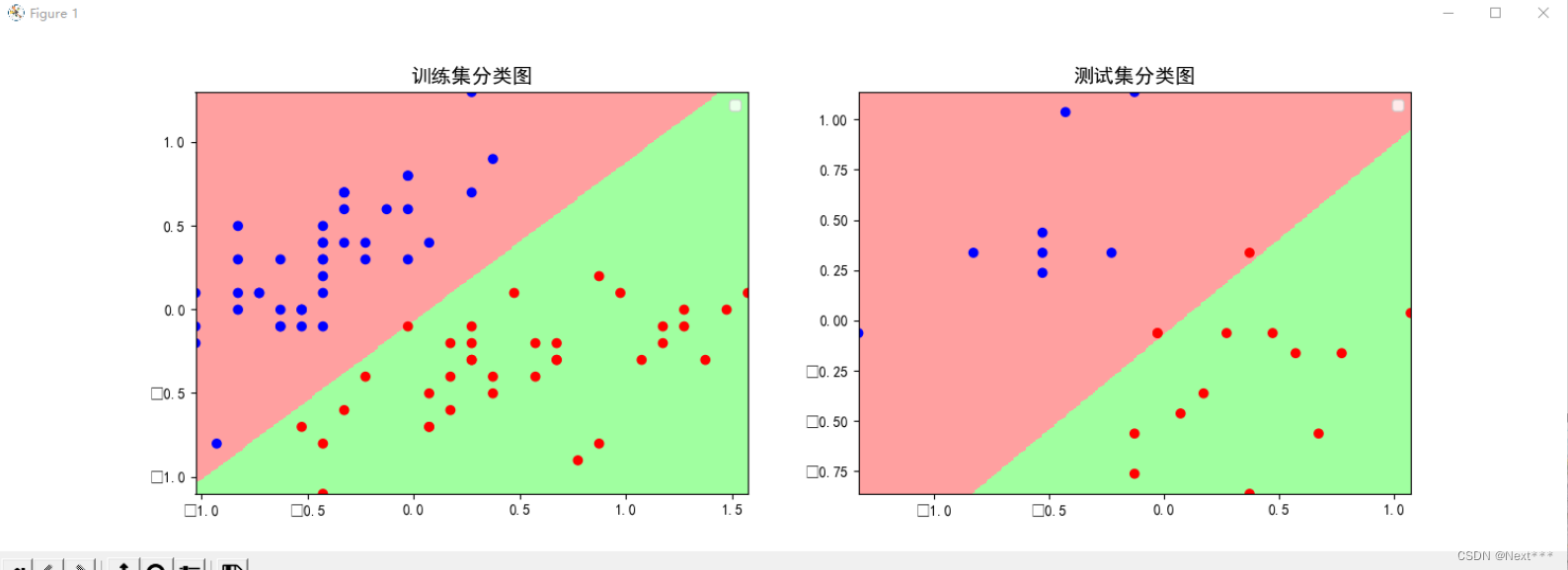
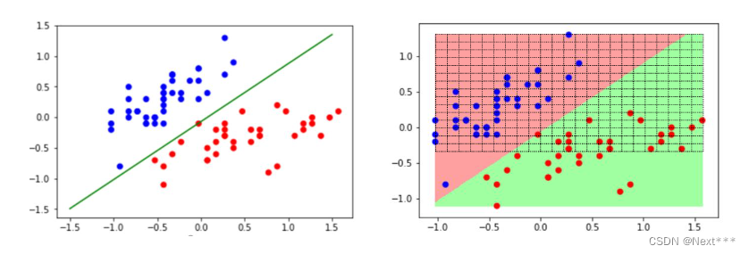
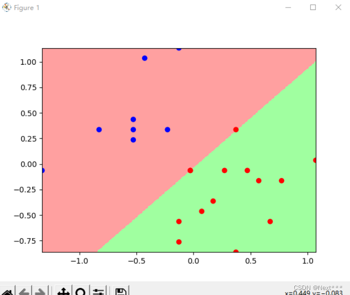
- 测试集上看着有两个分类错误,其实是三个,因为测试集里面有两个重合点
11.4.2.5 使用定义函数借鉴上一节代码
讨论【11.4】绘制测试集分类图
课程编程实例中,有很多代码是重复的,是否可以通过函数来实现代码复用?同学们尝试一下,并在讨论区分享关键代码,大家共同学习。
#加载数据
import tensorflow as tf
import numpy as np
import matplotlib as mpl
import matplotlib.pyplot as plt
import pandas as pd
from numpy.lib.function_base import disp#数据准备
def preparedData(URL):path=tf.keras.utils.get_file(URL.split('/')[-1],URL)df_iris=pd.read_csv(path,header=0)iris=np.array(df_iris)_x=iris[:,0:2]_y=iris[:,4]x=_x[_y<2]y=_y[_y<2]num=len(x)X,Y,x=dataCentralize(x,y,num)return X,Y,x,y#数据中心化
def dataCentralize(x,y,num):x=x-np.mean(x,axis=0)x0=np.ones(num).reshape(-1,1)X=tf.cast(tf.concat((x0,x),axis=1),tf.float32)Y=tf.cast(y.reshape(-1,1),tf.float32)return X,Y,x#获取导数
def getDerivate(X,Y,W,ce,acc,flag):with tf.GradientTape() as tape:PRED=1/(1+tf.exp(-tf.matmul(X,W)))Loss=-tf.reduce_mean(Y*tf.math.log(PRED)+(1-Y)*tf.math.log(1-PRED))accuracy=tf.reduce_mean(tf.cast(tf.equal(tf.where(PRED.numpy()<0.5,0.,1.),Y),tf.float32))ce.append(Loss)acc.append(accuracy)if  flag==1:dL_dW=tape.gradient(Loss,W)W.assign_sub(learn_rate*dL_dW)return ce,acc,W#绘图
def mapping(x,y):M=300x1_min,x2_min=x.min(axis=0)x1_max,x2_max=x.max(axis=0)t1=np.linspace(x1_min,x1_max,M)t2=np.linspace(x2_min,x2_max,M)m1,m2=np.meshgrid(t1,t2)m0=np.ones(M*M)X_mesh=tf.cast(np.stack((m0,m1.reshape(-1),m2.reshape(-1)),axis=1),dtype=tf.float32)Y_mesh=tf.cast(1/(1+tf.exp(-tf.matmul(X_mesh,W))),dtype=tf.float32)Y_mesh=tf.where(Y_mesh<0.5,0,1)n=tf.reshape(Y_mesh,m1.shape)cm_pt=mpl.colors.ListedColormap(["blue","red"])cm_bg=mpl.colors.ListedColormap(["#FFA0A0","#A0FFA0"])plt.pcolormesh(m1,m2,n,cmap=cm_bg)plt.scatter(x[:,0],x[:,1],c=y,cmap=cm_pt)plt.show()#数据加载
TRAIN_URL="https://download.tensorflow.org/data/iris_training.csv"
TEST_URL="https://download.tensorflow.org/data/iris_test.csv"
X_train,Y_train,x_train,y_train=preparedData(TRAIN_URL)
X_test,Y_test,x_test,y_test=preparedData(TEST_URL)#设置超参
learn_rate=0.2
iter=120
display_step=30#设置模型参数初始值
np.random.seed(612)
W=tf.Variable(np.random.randn(3,1),dtype=tf.float32)#训练模型
ce_train=[]
acc_train=[]
ce_test=[]
acc_test=[]for i in range(0,iter+1):acc_train,ce_train,W=getDerivate(X_train,Y_train,W,ce_train,acc_train,1)acc_test,ce_test,W=getDerivate(X_train,Y_train,W,ce_train,acc_train,1)if i % display_step==0:print("i:%i\tAcc:%f\tLoss:%f\tAcc_test:%f\tLoss_test:%f"%(i,acc_train[i],ce_train[i],acc_test[i],ce_test[i]))#绘图#x_train,y_train,
mapping(x_test,y_test)
输出结果为:
i:0     Acc:0.994269    Loss:0.230769   Acc_test:0.230769       Loss_test:0.994269
i:30    Acc:0.961538    Loss:0.481892   Acc_test:0.481892       Loss_test:0.961538
i:60    Acc:0.319128    Loss:0.987179   Acc_test:0.987179       Loss_test:0.319128
i:90    Acc:0.987179    Loss:0.246626   Acc_test:0.246626       Loss_test:0.987179
i:120   Acc:0.204982    Loss:1.000000   Acc_test:1.000000       Loss_test:0.204982
11.4.2.6 使用四种属性区分变色鸢尾和维吉尼亚鸢尾
鸢尾花数据集中,有四个属性(花瓣长度、花瓣宽度、花萼长度、花萼宽度),课程中只是给出了两种属性组合的情况,如果采用三种或者四种属性去训练模型,能否把变色鸢尾和维吉尼亚鸢尾完全区分开呢?请简要说明一下你用的哪几种属性并在讨论区晒出你的程序结果。
# 1 加载数据
import tensorflow as tf
import pandas as pd
import numpy as np
import matplotlib as mpl
import matplotlib.pyplot as pltTRAIN_URL = "http://download.tensorflow.org/data/iris_training.csv"
TEST_URL = "http://download.tensorflow.org/data/iris_test.csv"
train_path = tf.keras.utils.get_file(TRAIN_URL.split('/')[-1],TRAIN_URL)
test_path = tf.keras.utils.get_file(TEST_URL.split('/')[-1],TEST_URL)df_iris_train = pd.read_csv(train_path,header=0) # 是一个pandas二维数据表
df_iris_test =  pd.read_csv(test_path,header=0)# 2 处理数据
# 首先将二维数据表转化为numpy数组
iris_train= np.array(df_iris_train)  # shape(120,5)
iris_test= np.array(df_iris_test)  # shape(30,5)# 提取属性和标签
train_x = iris_train[:,0:4]  # (120,4)
train_y = iris_train[:,4] # (120,)test_x = iris_test[:,0:4]  # (30,4)
test_y = iris_test[:,4] # (30,)
# 提取山鸢尾和变色鸢尾,提取出标签纸为0和1的值
x_train = train_x[train_y > 0] # (n,4)
y_train = train_y[train_y > 0]-1 # (n,)x_test = test_x[test_y > 0] # (m,4)
y_test = test_y[test_y > 0]-1 # (m,)
# 记录现在的样本数
num_train = len(x_train)
num_test = len(x_test)
# 分别进行按列中心化处理,要求训练集和测试集独立同分布的,具有相同的均值和方差,数量有限的情况下,只要尽量接近即可
# 使用划分好的不用太考虑,但是自己划分数据集,要考虑这点x_train = x_train - np.mean(x_train,axis= 0)
x_test = x_test - np.mean(x_test,axis=0)# 生成多元模型的属性矩阵和标签列向量
x0_train = np.ones(num_train).reshape(-1,1)
X_train = tf.cast(tf.concat((x0_train,x_train),axis=1),tf.float32) # shape(n,5)
Y_train = tf.cast(y_train.reshape(-1,1),tf.float32) # shape(n,1)x0_test = np.ones(num_test).reshape(-1,1)
X_test = tf.cast(tf.concat((x0_test,x_test),axis=1),dtype=tf.float32) # (m,5)
Y_test = tf.cast(y_test.reshape(-1,1),dtype=tf.float32) # (m,1)# 3 设置超参数
learn_rate = 0.135
iter = 10000
display_step = 1000# 4 设置模型参数初始值
np.random.seed(612)
W = tf.Variable(np.random.randn(5,1),dtype=tf.float32)# 5 训练模型
ce_train = []
acc_train = []
ce_test = []
acc_test = []for i in range(0,iter+1):with tf.GradientTape() as tape:PRED_train = 1/(1+tf.exp(-tf.matmul(X_train,W))) # 每个样本的预测概率Loss_train = -tf.reduce_mean(Y_train*tf.math.log(PRED_train)+(1-Y_train)*tf.math.log(1-PRED_train))PRED_test = 1/(1+tf.exp(-tf.matmul(X_test,W))) # 每个样本的预测概率Loss_test = -tf.reduce_mean(Y_test*tf.math.log(PRED_test)+(1-Y_test)*tf.math.log(1-PRED_test))accuracy_train = tf.reduce_mean(tf.cast(tf.equal(tf.where(PRED_train.numpy()<0.5,0.,1.),Y_train),tf.float32))accuracy_test = tf.reduce_mean(tf.cast(tf.equal(tf.where(PRED_test.numpy()<0.5,0.,1.),Y_test),tf.float32))ce_train.append(Loss_train)acc_train.append(accuracy_train)ce_test.append(Loss_test)acc_test.append(accuracy_test)dL_dW = tape.gradient(Loss_train,W)W.assign_sub(learn_rate*dL_dW)if i % display_step ==0:print("i: %i, TrainAcc: %f, TrainLoss: %f, TestAcc: %f, TestLoss: %f" % (i,accuracy_train,Loss_train,accuracy_test,Loss_test))#可视化:绘制损失和准确率变化曲线
plt.figure(figsize=(10,3))
plt.subplot(121)
plt.plot(ce_train,color="blue",label="train")
plt.plot(ce_test,color="red",label="test")
plt.ylabel("Loss")
plt.legend()plt.subplot(122)
plt.plot(acc_train,color="blue",label="train")
plt.plot(acc_test,color="red",label="test")
plt.ylabel("Accuracy")
plt.legend()plt.show()
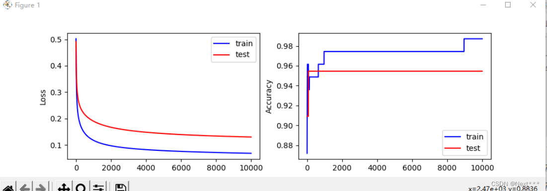
输出结果为:
i: 0, TrainAcc: 0.871795, TrainLoss: 0.502093, TestAcc: 0.909091, TestLoss: 0.491409
i: 1000, TrainAcc: 0.974359, TrainLoss: 0.117291, TestAcc: 0.954545, TestLoss: 0.189897
i: 2000, TrainAcc: 0.974359, TrainLoss: 0.096742, TestAcc: 0.954545, TestLoss: 0.166818
i: 3000, TrainAcc: 0.974359, TrainLoss: 0.087580, TestAcc: 0.954545, TestLoss: 0.155260
i: 4000, TrainAcc: 0.974359, TrainLoss: 0.082096, TestAcc: 0.954545, TestLoss: 0.148034
i: 5000, TrainAcc: 0.974359, TrainLoss: 0.078296, TestAcc: 0.954545, TestLoss: 0.142953
i: 6000, TrainAcc: 0.974359, TrainLoss: 0.075425, TestAcc: 0.954545, TestLoss: 0.139118
i: 7000, TrainAcc: 0.974359, TrainLoss: 0.073129, TestAcc: 0.954545, TestLoss: 0.136092
i: 8000, TrainAcc: 0.974359, TrainLoss: 0.071221, TestAcc: 0.954545, TestLoss: 0.133636
i: 9000, TrainAcc: 0.987179, TrainLoss: 0.069592, TestAcc: 0.954545, TestLoss: 0.131605
i: 10000, TrainAcc: 0.987179, TrainLoss: 0.068172, TestAcc: 0.954545, TestLoss: 0.129906
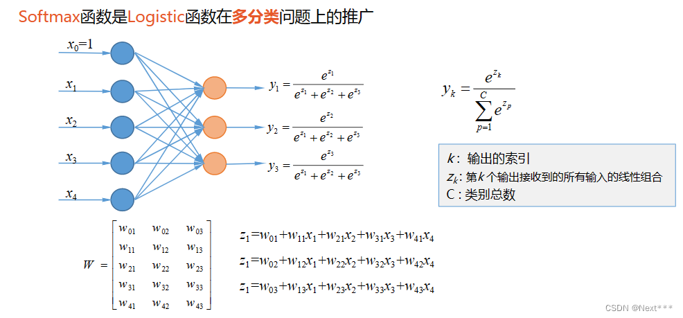
11.5 多分类问题
- 逻辑回归:二分类问题
- 多分类问题:把输入样本划分为多个类别
- 下面以鸢尾花为例,实现多分类类别
11.5.1 类别编码问题
-
自然顺序码
0 —— 山鸢尾(Setosa)
1 —— 变色鸢尾(Versicolour)
2 —— 维吉尼亚鸢尾(Virginica)
欧氏距离使得类别之间不平等,但是实际上类别之间应该是平等的 -
独热编码(One-Hot Encoding)
使非偏序关系的数据,取值不具有偏序性
到原点等距
(1,0,0) —— 山鸢尾(Setosa)
(0,1,0) —— 变色鸢尾(Versicolour)
(0,0,1) —— 维吉尼亚鸢尾(Virginica)
需要占用更多的空间,但是能够更加合理的表示数据之间的关系,可以有效的避免学习中的偏差 -
独热的 应用
离散的特征
多分类问题中的类别标签 -
独冷编码(One-Hot Encoding)
(0,1,1) —— 山鸢尾(Setosa)
(1,0,1) —— 变色鸢尾(Versicolour)
(1,1,0) —— 维吉尼亚鸢尾(Virginica)
11.5.2 实例,多分类问题
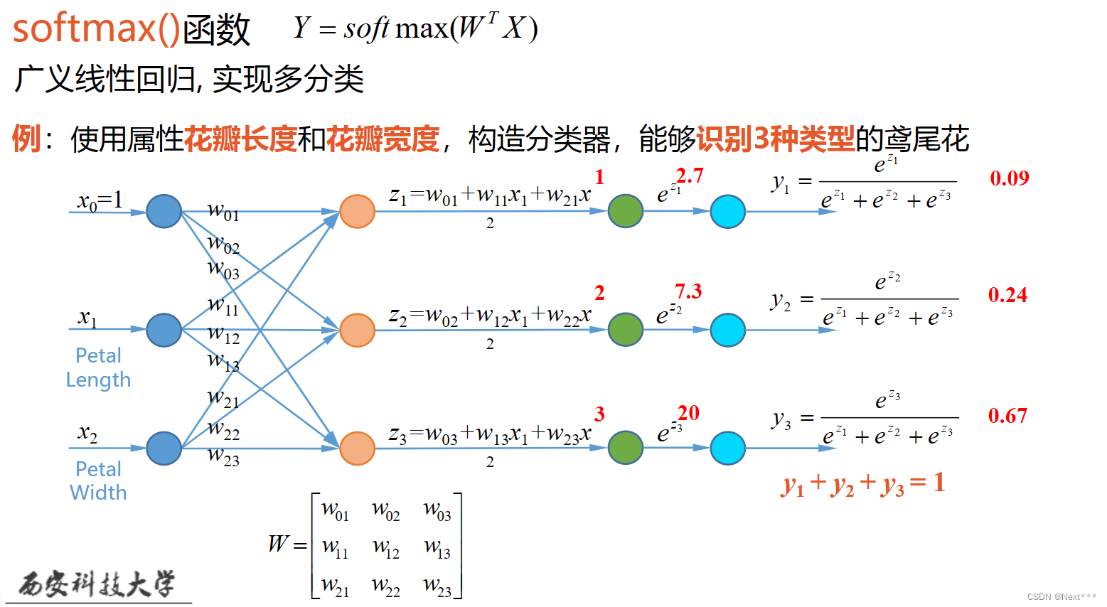
- 例:使用属性花瓣长度和花瓣宽度,构造分类器,能够识别3种类型的鸢尾花
-
互斥的多分类问题:每个样本只能够属于一个类别
鸢尾花的识别
手写数字的识别 -
标签:一个图片可以被打上多个标签,即一个样本可以同时属于多个类别
彩色图片
包括人物的图片
包括汽车的图片
户外图片
室内图片
11.6 实例:多分类问题
11.6.1 独热编码的实现
tf.one_hot(indices,depth)
- indices:一维数组/张量
- depth:编码深度,也就是分成几类
>>> import tensorflow as tf
>>> print(tf.__version__)
2.0.0
>>> import numpy as np
>>> a = [0,2,3,5]
>>> b = tf.one_hot(a,6)
>>> b
<tf.Tensor: id=9, shape=(4, 6), dtype=float32, numpy=
array([[1., 0., 0., 0., 0., 0.],[0., 0., 1., 0., 0., 0.],[0., 0., 0., 1., 0., 0.],[0., 0., 0., 0., 0., 1.]], dtype=float32)>
11.6.2 准确率的计算
# 预测值
>>> pred = np.array([[0.1,0.2,0.7],[0.1,0.7,0.2],[0.3,0.4,0.3]])
# 标记
>>> y = np.array([2,1,0])
# 标记独热编码
>>> y_onehot = np.array([[0,0,1],[0,1,0],[1,0,0]])
# 预测值中的最大数索引
>>> tf.argmax(pred,axis=1)
<tf.Tensor: id=12, shape=(3,), dtype=int64, numpy=array([2, 1, 1], dtype=int64)>
# 判读预测值是否与样本标记相同
>>> tf.equal(tf.argmax(pred,axis=1),y)
<tf.Tensor: id=17, shape=(3,), dtype=bool, numpy=array([ True,  True, False])>
# 将布尔值转化为数字
>>> tf.cast(tf.equal(tf.argmax(pred,axis=1),y),tf.float32)
<tf.Tensor: id=23, shape=(3,), dtype=float32, numpy=array([1., 1., 0.], dtype=float32)>
# 计算准确率
>>> tf.reduce_mean(tf.cast(tf.equal(tf.argmax(pred,axis=1),y),tf.float32))
<tf.Tensor: id=39, shape=(), dtype=float32, numpy=0.6666667>
11.6.3 交叉熵损失函数的实现
代码接11.6.2
>>> -y_onehot*tf.math.log(pred)
<tf.Tensor: id=43, shape=(3, 3), dtype=float64, numpy=
array([[-0.        , -0.        ,  0.35667494],       [-0.        ,  0.35667494, -0.        ],       [ 1.2039728 , -0.        , -0.        ]])>
# 所有样本交叉熵之和
>>> -tf.reduce_sum(y_onehot*tf.math.log(pred))
<tf.Tensor: id=50, shape=(), dtype=float64, numpy=1.917322692203401>
# 平均交叉熵损失
>>> -tf.reduce_sum(y_onehot*tf.math.log(pred))/len(pred)
<tf.Tensor: id=59, shape=(), dtype=float64, numpy=0.6391075640678003>
>>> len(pred)
3
11.6.4 使用花瓣长度、花瓣宽度将三种鸢尾花区分开
11.6.4.0 修改动态分配显存(空)
11.6.4.1 加载数据
# 1 加载数据
import tensorflow as tf
import pandas as pd
import numpy as np
import matplotlib as mpl
import matplotlib.pyplot as plt
# 修改配置-动态分配显存
gpus = tf.config.experimental.list_physical_devices(device_type='GPU')
tf.config.experimental.set_memory_growth(gpus[0], True)TRAIN_URL = "http://download.tensorflow.org/data/iris_training.csv"
TEST_URL = "http://download.tensorflow.org/data/iris_test.csv"train_path = tf.keras.utils.get_file(TRAIN_URL.split('/')[-1],TRAIN_URL)
test_path = tf.keras.utils.get_file(TEST_URL.split('/')[-1],TEST_URL)df_iris_train = pd.read_csv(train_path, header=0)
11.6.4.2 处理数据
# 2 处理数据
iris_train = np.array(df_iris_train)
# (120,5)#提取花瓣长度、花瓣宽度属性
x_train = iris_train[:,2:4]
# (120,2)
y_train = iris_train[:,4]
# (120,)num_train = len(x_train)x0_train = np.ones(num_train).reshape(-1,1)
X_train = tf.cast(tf.concat([x0_train,x_train],axis=1),tf.float32)
# ([120,3])
Y_train = tf.one_hot(tf.constant(y_train,dtype=tf.int32),3)
# ([120,3])
11.6.4.3 设置超参数、设置模型参数初始值
# 3 设置超参数、设置模型参数初始值
learn_rate = 0.2
iter = 500
display_step = 100np.random.seed(612)
W = tf.Variable(np.random.randn(3,3),dtype=tf.float32)
11.6.4.4 训练模型
# 4 训练模型
acc = []
cce = []for i in range(0,iter+1):with tf.GradientTape() as tape:# (120,3) 属于每种类别的概率,每个样本三种类别概率之和为1PRED_train = tf.nn.softmax(tf.matmul(X_train,W))Loss_train = -tf.reduce_sum(Y_train*tf.math.log(PRED_train))/num_trainaccuracy = tf.reduce_mean(tf.cast(tf.equal(tf.argmax(PRED_train.numpy(),axis=1),y_train),tf.float32))acc.append(accuracy)cce.append(Loss_train)dL_dW = tape.gradient(Loss_train,W)W.assign_sub(learn_rate*dL_dW)if i % display_step == 0:print("i: %i, Acc: %f, Loss: %f"%(i,accuracy,Loss_train))
输出结果为:
i: 0, Acc: 0.350000, Loss: 4.510763
i: 100, Acc: 0.808333, Loss: 0.503537
i: 200, Acc: 0.883333, Loss: 0.402912
i: 300, Acc: 0.891667, Loss: 0.352650
i: 400, Acc: 0.941667, Loss: 0.319778
i: 500, Acc: 0.941667, Loss: 0.295599
11.6.4.5 查看训练结果
# 5 查看训练结果
# 输出自然顺序码
print("自然顺序码为:" )
print(tf.argmax(PRED_train.numpy(),axis=1))
``
输出结果为:```python
自然顺序码为:
tf.Tensor(
[2 1 2 0 0 0 0 2 1 0 1 1 0 0 2 2 2 2 2 0 2 2 0 1 1 0 1 2 1 2 1 1 1 2 2 2 22 0 0 2 2 2 0 0 1 0 2 0 2 0 1 1 0 1 2 2 2 2 1 1 2 2 2 1 2 0 2 2 0 0 1 0 22 0 1 1 1 2 0 1 1 1 2 0 1 1 2 0 2 1 0 0 2 0 0 2 2 0 0 1 0 1 0 0 0 0 1 0 21 0 2 0 1 1 0 0 1], shape=(120,), dtype=int64)
11.6.4.6 绘制分类图
# 6 绘制分类图
M = 500
x1_min,x2_min = x_train.min(axis=0)
x1_max,x2_max = x_train.max(axis=0)
t1 = np.linspace(x1_min,x1_max,M)
t2 = np.linspace(x2_min,x2_max,M)
m1,m2 = np.meshgrid(t1,t2)m0 = np.ones(M*M)
X_ = tf.cast(np.stack((m0,m1.reshape(-1),m2.reshape(-1)),axis=1),tf.float32)
Y_ = tf.nn.softmax(tf.matmul(X_,W))Y_ = tf.argmax(Y_.numpy(),axis=1)# 转换为自然顺序码n = tf.reshape(Y_,m1.shape)# (500,500)plt.figure(figsize = (8,6))
cm_bg =  mpl.colors.ListedColormap(['#A0FFA0','#FFA0A0','#A0A0FF'])plt.pcolormesh(m1,m2,n,cmap=cm_bg)
plt.scatter(x_train[:,0],x_train[:,1],c = y_train,cmap="brg")plt.show()
11.6.4.7 本例代码汇总
# 1 加载数据
import tensorflow as tf
import pandas as pd
import numpy as np
import matplotlib as mpl
import matplotlib.pyplot as pltgpus = tf.config.experimental.list_physical_devices(device_type='GPU')
tf.config.experimental.set_memory_growth(gpus[0], True)TRAIN_URL = "http://download.tensorflow.org/data/iris_training.csv"
TEST_URL = "http://download.tensorflow.org/data/iris_test.csv"train_path = tf.keras.utils.get_file(TRAIN_URL.split('/')[-1],TRAIN_URL)
test_path = tf.keras.utils.get_file(TEST_URL.split('/')[-1],TEST_URL)df_iris_train = pd.read_csv(train_path, header=0)# 2 处理数据
iris_train = np.array(df_iris_train)
# (120,5)#提取花瓣长度、花瓣宽度属性
x_train = iris_train[:,2:4]
# (120,2)
y_train = iris_train[:,4]
# (120,)num_train = len(x_train)x0_train = np.ones(num_train).reshape(-1,1)
X_train = tf.cast(tf.concat([x0_train,x_train],axis=1),tf.float32)
# ([120,3])
Y_train = tf.one_hot(tf.constant(y_train,dtype=tf.int32),3)
# ([120,3])# 3 设置超参数、设置模型参数初始值
learn_rate = 0.2
iter = 500
display_step = 100np.random.seed(612)
W = tf.Variable(np.random.randn(3,3),dtype=tf.float32)# 4 训练模型
acc = []
cce = []for i in range(0,iter+1):with tf.GradientTape() as tape:PRED_train = tf.nn.softmax(tf.matmul(X_train,W))# (120,3) 属于每种类别的概率,每个样本三种类别概率之和为1Loss_train = -tf.reduce_sum(Y_train*tf.math.log(PRED_train))/num_trainaccuracy = tf.reduce_mean(tf.cast(tf.equal(tf.argmax(PRED_train.numpy(),axis=1),y_train),tf.float32))acc.append(accuracy)cce.append(Loss_train)dL_dW = tape.gradient(Loss_train,W)W.assign_sub(learn_rate*dL_dW)if i % display_step == 0:print("i: %i, Acc: %f, Loss: %f"%(i,accuracy,Loss_train))# 5 查看训练结果
# 输出自然顺序码
print("自然顺序码为:" )
print(tf.argmax(PRED_train.numpy(),axis=1))# 6 绘制分类图
M = 500
x1_min,x2_min = x_train.min(axis=0)
x1_max,x2_max = x_train.max(axis=0)
t1 = np.linspace(x1_min,x1_max,M)
t2 = np.linspace(x2_min,x2_max,M)
m1,m2 = np.meshgrid(t1,t2)m0 = np.ones(M*M)
X_ = tf.cast(np.stack((m0,m1.reshape(-1),m2.reshape(-1)),axis=1),tf.float32)
Y_ = tf.nn.softmax(tf.matmul(X_,W))Y_ = tf.argmax(Y_.numpy(),axis=1)# 转换为自然顺序码n = tf.reshape(Y_,m1.shape)# (500,500)plt.figure(figsize = (8,6))
cm_bg =  mpl.colors.ListedColormap(['#A0FFA0','#FFA0A0','#A0A0FF'])plt.pcolormesh(m1,m2,n,cmap=cm_bg)
plt.scatter(x_train[:,0],x_train[:,1],c = y_train,cmap="brg")plt.show()
【参考文献】: 神经网络与深度学习——TensorFlow实践
相关文章:
Lesson11---分类问题
11.1 逻辑回归 11.1.1 广义线性回归 课程回顾 线性回归:将自变量和因变量之间的关系,用线性模型来表示;根据已知的样本数据,对未来的、或者未知的数据进行估计 11.1.2 逻辑回归 11.1.2.1 分类问题 分类问题:垃圾…...

Python基础学习12——异常
在Python中,会使用“异常”这个十分特殊的对象来管理程序执行期间发生的错误,即报错。本文将介绍一下python基础的处理异常的方法以及一些基本的异常类型。 异常处理方法 try-except代码块 当我们编写程序时,我们可以编写一个try-except代…...

[日常练习]练习17:链表头插法、尾插法练习
[日常练习]练习17:链表头插法、尾插法练习练习17描述输入输出输入示例1输出示例1输入示例2输出示例2代码演示:总结练习17 【日常练习】 链表头插法、尾插法练习 描述 输入3 4 5 6 7 9999一串整数,9999代表结束,通过头插法新建链…...
第十四届蓝桥杯模拟赛(第三期)试题与题解 C++
目录 一、填空题 (一)最小的十六进制(答案:2730) (二)Excel的列(答案:BYT) (三)相等日期(答案:70910) (四)多少种取法(答案:189)…...

关于 “宏“
起源 宏 Macro"这个词源于希腊语 “makros”,意为“大的,长的” 延伸使用 随后用于计算机领域是,在汇编语言时用于描述一大堆的汇编指令。 只要用宏指令,就是直接用的一大堆的汇编指令(有点函数的味道…...

1.2 CSS标签选择器,类选择器
CSS选择器: 根据不同的需求选出不同的标签,进行美化装饰 1. 标签选择器 标签选择器(元素选择器):用 HTML标签名作为选择器,按标签名称进行分类,为页面某一类标签指定统一的CSS样式 作用: 可以把某一类标签全部选中&…...

【Linux】进程等待 | 详解 wait/waitpid 的 status 参数
🤣 爆笑教程 👉 《看表情包学Linux》👈 猛戳订阅 🔥 💭 写在前面:在上一章中我们讲解了进程创建与进程终止,本章我们开始讲解进程等待。进程等待这部分知识相较于前面还是较为复杂的࿰…...

OpenAI眼中的无线调优策略
问:无线调优策略该怎么优化无线调优是指对无线网络的各种参数进行优化,以提高网络性能和用户体验。以下是几个无线调优策略:频谱分配:通过优化频谱的分配,可以提高网络的容量和覆盖范围。在频谱分配时,需要…...
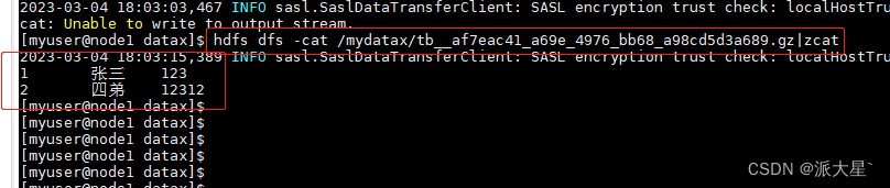
DataX入门
目录 1. DataX介绍 2. DataX支持的常用数据源类型 3. 设计理念 4. DataX框架设计 4.1. Reader 4.2. Writer 4.3. Framework 5. DataX的运行流程 6. DataX与Sqoop对比 7. 部署 8. 配置详解 9. 案例 同步MySql到HDFS 9.1. 整体结构 9.2. mySqlReader 9.2.1. …...

第二章SpringBoot基础学习
文章目录SpringBoot依赖管理特性依赖管理开发导入starter场景启动器SpringBoot自动配置特性自动配好Tomcat自动配好SpringMVC默认的包结构各种配置拥有默认值按需加载所有自动配置项SpringBoot注解底层注解ConfigurationImport导入组件Conditional条件装配ImportResource导入Sp…...
B - Build Roads (最小生成树 + 打表)
https://vjudge.net/problem/Gym-103118B/origin 在猫的国度里,有n个城市。猫国国王想要修n -1条路来连接所有的城市。第i市有一家ai经验价值的建筑公司。要在第i市和第j市之间修建公路,两个城市的建筑公司需要相互合作。但是,在修路的过程中…...

k8s管理工具
k8s管理工具 文章目录k8s管理工具Kuboard(💕17.3k)KubeOperator(💕4.6k)Rainbond(💕3.8k)KubeSphere(💕12k)Kuboard(&…...

Cannot start compiler The output path is not specified for module mystatic(已解决)
1.背景:今天在idea上写了一些代码,右键run竟然跑不起来了,而且右下角的Event Log还报错。报错内容如下图:2.报错原因:项目代码和编译器的输出路径不在一块,导致idea无法找到模块的output path(输…...

python入门应该怎么学习
国外Python的使用率非常高,但在国内Python是近几年才火起来,Python正处于高速上升期市场对于Python开发人才的需求量急剧增加,学习Python的前景比较好。 Python应用领域广泛,意味着选择Python的同学在学成之后可选择的就业领域有…...

不懂命令, 如何将代码托管到Gitee上
1.注册码云注册地址 : https://gitee.com2. 新建仓库第一步 : 创建仓库第二步 : 给仓库起名字创建好仓库后, 我们就有了一个网络上的仓库 : 3. 将网络上的仓库克隆到本地在克隆仓库之前, 我们需要先在电脑上安装以下两个工具 >>这两个软件一定要按顺序安装, 先安装第一个…...
Mysql常见面试题总结
1、什么是存储引擎 存储引擎指定了表的类型,即如何存储和索引数据,是否支持事务,同时存储引擎也决定了表在计算机中的存储方式。 2、查看数据库支持哪些存储引擎使用什么命令? -- 查看数据库支持的存储引擎 show engines; 或者 …...

python第一周作业
作业1:1、PPT上五个控制台界面2、要求定义两个数,并且交换它们的值(请使用多种方式,越多越好)作业1作业2:判断一个数,是否是2的指数2的指数0000 0010 0000 00010000 0100 0000 00110000 1000 00…...
FLoyd算法的入门与应用
目录 一、前言 二、FLoyd算法 1、最短路问题 2、Floyd算法 3、Floyd的特点 4、Floyd算法思想:动态规划 三、例题 1、蓝桥公园(lanqiaoOJ题号1121) 2、路径(2021年初赛 lanqiaoOJ题号1460) 一、前言 本文主要…...
303. 区域和检索 - 数组不可变
303. 区域和检索 - 数组不可变 给定一个整数数组 nums,处理以下类型的多个查询: 计算索引 left 和 right (包含 left 和 right)之间的 nums 元素的 和 ,其中 left < right 实现 NumArray 类: NumArray(int[] num…...
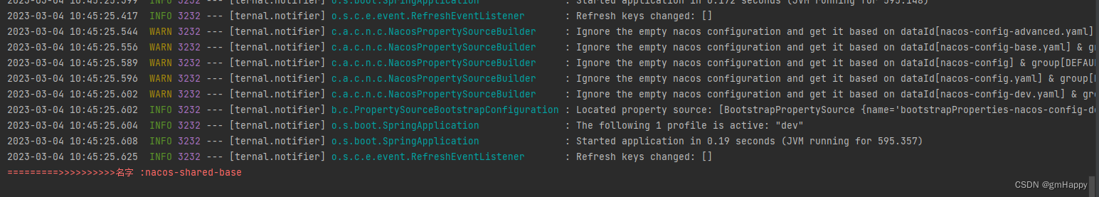
Spring Cloud融合Nacos配置加载优先级 | Spring Cloud 8
一、前言 Spring Cloud Alibaba Nacos Config 目前提供了三种配置能力从 Nacos 拉取相关的配置: A:通过内部相关规则(应用名、扩展名、profiles)自动生成相关的 Data Id 配置B:通过 spring.cloud.nacos.config.extension-configs的方式支持…...

python confluence
# Python Confluence:让团队知识流动起来 在团队协作中,知识管理常常是个令人头疼的问题。文档散落在各处,版本混乱,新成员找不到关键信息,老员工的经验难以沉淀。如果你也遇到过这些问题,那么Python Conf…...

如何快速解决Hackintosh配置难题:OpCore-Simplify终极解决方案指南
如何快速解决Hackintosh配置难题:OpCore-Simplify终极解决方案指南 【免费下载链接】OpCore-Simplify A tool designed to simplify the creation of OpenCore EFI 项目地址: https://gitcode.com/GitHub_Trending/op/OpCore-Simplify 还在为复杂的OpenCore …...

vLLM-v0.17.1步骤详解:支持LoRA热切换的动态模型服务配置
vLLM-v0.17.1步骤详解:支持LoRA热切换的动态模型服务配置 1. vLLM框架简介 vLLM是一个专为大型语言模型(LLM)设计的高性能推理和服务库,以其出色的吞吐量和易用性著称。这个项目最初由加州大学伯克利分校的天空计算实验室开发,现在已经发展…...
)
新手避坑指南:用STC AI8051U和GPS搞定智能车气垫越野组(附完整代码)
智能车竞赛气垫越野组实战指南:从零搭建到精准导航 1. 初识气垫越野组:竞赛特点与技术挑战 智能车竞赛气垫越野组是近年来最富挑战性的组别之一,它要求参赛车辆在完全依靠气垫推进的情况下,自主完成室外复杂地形的导航任务。与传统…...

客户决策链地图怎么画:老板、采购、技术、项目、法务分别怎么看你
在很多B2B企业的表达体系里,“客户”这个词经常被用得过于整齐。 官网会写“服务行业客户”,销售会说“面向大型企业”,PPT会写“解决复杂需求”。这些话都没问题,但它们通常默认一个前提:客户像一个人一样在决策。而真…...

OpenClaw技能开发入门:为Phi-3-vision制作商品截图分析插件
OpenClaw技能开发入门:为Phi-3-vision制作商品截图分析插件 1. 为什么需要商品截图分析技能 上周我在整理双十一购物清单时,发现手动对比不同平台的商品价格和促销信息简直是一场噩梦。每次都要反复截图、整理、记录,效率低下还容易出错。这…...

the-glorious-dotfiles 核心功能解析:从通知中心到屏幕录制
the-glorious-dotfiles 核心功能解析:从通知中心到屏幕录制 【免费下载链接】the-glorious-dotfiles A glorified personal dot files 项目地址: https://gitcode.com/gh_mirrors/th/the-glorious-dotfiles the-glorious-dotfiles 是一套功能丰富的个人配置文…...

eksctl多集群管理终极指南:跨区域部署和统一运维实践
eksctl多集群管理终极指南:跨区域部署和统一运维实践 【免费下载链接】eksctl The official CLI for Amazon EKS 项目地址: https://gitcode.com/gh_mirrors/ek/eksctl eksctl作为Amazon EKS官方CLI工具,为用户提供了快速创建、管理和运维Kuberne…...

为什么头部自动驾驶团队已在预研C++27反射?——静态反射在嵌入式ABI稳定、安全认证代码生成中的不可替代性揭秘
第一章:C27静态反射的演进脉络与战略定位C27静态反射并非凭空而生,而是ISO C标准化进程中长达十年深度探索的结晶。它继承并重构了C17的std::is_same、C20的std::source_location与反射TS(P0194R8)的语义骨架,同时彻底…...

2025最权威的六大降AI率方案推荐榜单
Ai论文网站排名(开题报告、文献综述、降aigc率、降重综合对比) TOP1. 千笔AI TOP2. aipasspaper TOP3. 清北论文 TOP4. 豆包 TOP5. kimi TOP6. deepseek 减少AIGC(人工智能生成内容)的痕迹,要从多方面入手&…...