差分矩阵(Difference Matrix)与累计和矩阵(Running Sum Matrix)的概念与应用:中英双语
本文是学习这本书的笔记: https://web.stanford.edu/~boyd/vmls/
差分矩阵(Difference Matrix)与累计和矩阵(Running Sum Matrix)的概念与应用
在线性代数和信号处理等领域中,矩阵运算常被用来表示和计算各种数据变换。其中,差分矩阵(Difference Matrix)和累计和矩阵(Running Sum Matrix)是两个非常重要且有用的工具。它们可以高效地实现差分操作和累计和操作,在实际应用中非常广泛。本文将介绍这两个矩阵的定义、性质以及实际应用场景。
一、差分矩阵(Difference Matrix)
1. 定义
差分矩阵 ( D D D ) 是一个维度为 ( ( n − 1 ) × n (n-1) \times n (n−1)×n) 的稀疏矩阵,其形式如下:
D = [ − 1 1 0 ⋯ 0 0 0 − 1 1 ⋯ 0 0 ⋮ ⋮ ⋮ ⋱ ⋮ ⋮ 0 0 0 ⋯ − 1 1 ] . D = \begin{bmatrix} -1 & 1 & 0 & \cdots & 0 & 0 \\ 0 & -1 & 1 & \cdots & 0 & 0\\ \vdots & \vdots & \vdots & \ddots & \vdots & \vdots \\ 0 & 0 & 0 & \cdots & -1 & 1 \end{bmatrix}. D= −10⋮01−1⋮001⋮0⋯⋯⋱⋯00⋮−100⋮1 .
矩阵 ( D D D ) 的作用是对向量 ( x x x ) 计算相邻元素的差分,得到一个新的 ( ( n − 1 ) (n-1) (n−1))-维向量:
D x = [ x 2 − x 1 x 3 − x 2 ⋮ x n − x n − 1 ] . Dx = \begin{bmatrix} x_2 - x_1 \\ x_3 - x_2 \\ \vdots \\ x_n - x_{n-1} \end{bmatrix}. Dx= x2−x1x3−x2⋮xn−xn−1 .
2. 性质
- 稀疏性:差分矩阵中非零元素仅位于主对角线和次对角线上,计算效率高。
- 线性变换:差分操作可以被看作是一种线性变换,易于在矩阵计算框架中实现。
3. 实际应用
-
信号处理:
在信号处理中,差分矩阵可用来提取信号的变化趋势。例如,差分矩阵可以计算股票价格序列的每日变化(即价格增量):- 假设 ( x = [ 100 , 102 , 101 , 105 ] x = [100, 102, 101, 105] x=[100,102,101,105] ) 表示一段时间的股票价格,
- 通过 ( D D D ),可以计算价格增量为 ( D x = [ 2 , − 1 , 4 ] Dx = [2, -1, 4] Dx=[2,−1,4] )。
-
图像处理:
在图像处理中,差分矩阵可用于计算图像边缘信息。例如,针对一维图像信号,使用差分矩阵可以快速检测信号中的边缘变化。 -
优化问题:
在某些优化问题中,差分矩阵可以用来定义平滑性约束。例如,在路径规划中,约束路径的相邻点不能有过大的变化。
二、累计和矩阵(Running Sum Matrix)
1. 定义
累计和矩阵 ( S S S ) 是一个维度为 ( n × n n \times n n×n ) 的三角矩阵,其形式如下:
S = [ 1 0 0 ⋯ 0 1 1 0 ⋯ 0 1 1 1 ⋯ 0 ⋮ ⋮ ⋮ ⋱ 0 1 1 1 ⋯ 1 ] . S = \begin{bmatrix} 1 & 0 & 0 & \cdots & 0 \\ 1 & 1 & 0 & \cdots & 0 \\ 1 & 1 & 1 & \cdots & 0 \\ \vdots & \vdots & \vdots & \ddots & 0 \\ 1 & 1 & 1 & \cdots & 1 \end{bmatrix}. S= 111⋮1011⋮1001⋮1⋯⋯⋯⋱⋯00001 .
矩阵 ( S S S ) 的作用是对向量 ( x x x ) 计算累计和,得到一个新的 ( n n n)-维向量:
S x = [ x 1 x 1 + x 2 x 1 + x 2 + x 3 ⋮ x 1 + x 2 + ⋯ + x n ] . Sx = \begin{bmatrix} x_1 \\ x_1 + x_2 \\ x_1 + x_2 + x_3 \\ \vdots \\ x_1 + x_2 + \cdots + x_n \end{bmatrix}. Sx= x1x1+x2x1+x2+x3⋮x1+x2+⋯+xn .
2. 性质
- 稀疏性较弱:虽然矩阵 ( S S S ) 是稀疏的,但其三角的非零元素数量较多,相比差分矩阵稍显密集。
- 单调性:累计和是单调增加的,适用于需要累积计算的场景。
3. 实际应用
-
统计学分析:
在统计分析中,累计和常被用于计算数据的累积分布。例如,在处理时间序列数据时,可以用累计和来计算某个时间点之前的总和或平均值。 -
积分运算:
在离散数学中,累计和矩阵的作用类似于积分。对于一个离散信号 ( x x x ),累计和可以看作是该信号的离散积分。 -
金融数据分析:
在财务分析中,累计和矩阵可以用来计算累计收益。例如:- 假设 ( x = [ 10 , 15 , − 5 , 20 ] x = [10, 15, -5, 20] x=[10,15,−5,20] ) 表示每天的收益,
- 通过 ( S S S ),可以得到累计收益为 ( S x = [ 10 , 25 , 20 , 40 ] Sx = [10, 25, 20, 40] Sx=[10,25,20,40] )。
-
机器学习和深度学习:
在一些自然语言处理任务中(如Transformer模型中的注意力机制),累计和操作可以用于优化复杂的序列计算。
三、差分矩阵与累计和矩阵的关系
差分矩阵和累计和矩阵是互补的运算:
- 差分矩阵 ( D D D ) 的作用是从原始信号中提取增量信息;
- 累计和矩阵 ( S S S ) 的作用是从增量信息中重建累计值。
在数学上,它们满足如下关系:
D S = I n − 1 , DS = I_{n-1}, DS=In−1,
其中 ( I n − 1 I_{n-1} In−1 ) 是一个 ( ( n − 1 ) × ( n − 1 ) (n-1) \times (n-1) (n−1)×(n−1)) 的单位矩阵。这表明,差分矩阵 ( D D D ) 和累计和矩阵 ( S ) 是彼此的逆运算(在一定条件下)。
四、实际案例
案例:股票价格分析
假设有以下股票价格数据:
x = [ 100 102 101 105 ] . x = \begin{bmatrix} 100 \\ 102 \\ 101 \\ 105 \end{bmatrix}. x= 100102101105 .
-
计算每日价格增量:
使用差分矩阵 ( D D D ):
D = [ − 1 1 0 0 0 − 1 1 0 0 0 − 1 1 ] , D = \begin{bmatrix} -1 & 1 & 0 & 0 \\ 0 & -1 & 1 & 0 \\ 0 & 0 & -1 & 1 \end{bmatrix}, D= −1001−1001−1001 ,
计算:
D x = [ 2 − 1 4 ] . Dx = \begin{bmatrix} 2 \\ -1 \\ 4 \end{bmatrix}. Dx= 2−14 . -
计算累计收益:
使用累计和矩阵 ( S S S ):
S = [ 1 0 0 0 1 1 0 0 1 1 1 0 1 1 1 1 ] , S = \begin{bmatrix} 1 & 0 & 0 & 0 \\ 1 & 1 & 0 & 0 \\ 1 & 1 & 1 & 0 \\ 1 & 1 & 1 & 1 \end{bmatrix}, S= 1111011100110001 ,
计算:
S x = [ 100 202 303 408 ] . Sx = \begin{bmatrix} 100 \\ 202 \\ 303 \\ 408 \end{bmatrix}. Sx= 100202303408 .
五、总结
差分矩阵和累计和矩阵是两个非常有用的线性代数工具,在信号处理、统计分析、图像处理和金融分析等领域有广泛应用。差分矩阵用于提取相邻元素的增量信息,而累计和矩阵则用于计算累积值。通过这两个工具的结合,可以高效地完成各种线性变换和数据分析任务。
英文版
Difference Matrix and Running Sum Matrix: Concepts and Applications
In linear algebra and data processing, matrix operations are frequently used to represent and compute various transformations. Two important tools in this context are the Difference Matrix and the Running Sum Matrix. These matrices provide efficient ways to perform difference operations and cumulative sum operations, respectively, and have wide-ranging applications in real-world scenarios. This blog will introduce the definitions, properties, and applications of these two matrices.
1. Difference Matrix
Definition
The Difference Matrix ( D D D ) is a sparse matrix of size ( ( n − 1 ) × n (n-1) \times n (n−1)×n) with the following structure:
D = [ − 1 1 0 ⋯ 0 0 0 − 1 1 ⋯ 0 0 ⋮ ⋮ ⋮ ⋱ ⋮ ⋮ 0 0 0 ⋯ − 1 1 ] . D = \begin{bmatrix} -1 & 1 & 0 & \cdots & 0 & 0 \\ 0 & -1 & 1 & \cdots & 0 & 0\\ \vdots & \vdots & \vdots & \ddots & \vdots & \vdots \\ 0 & 0 & 0 & \cdots & -1 & 1 \end{bmatrix}. D= −10⋮01−1⋮001⋮0⋯⋯⋱⋯00⋮−100⋮1 .
The matrix ( D D D ) is used to compute the differences between consecutive elements of a vector ( x x x ). For an input vector ( x x x ), the output ( D x Dx Dx ) is an ( ( n − 1 ) (n-1) (n−1))-dimensional vector containing these differences:
D x = [ x 2 − x 1 x 3 − x 2 ⋮ x n − x n − 1 ] . Dx = \begin{bmatrix} x_2 - x_1 \\ x_3 - x_2 \\ \vdots \\ x_n - x_{n-1} \end{bmatrix}. Dx= x2−x1x3−x2⋮xn−xn−1 .
Properties
- Sparsity: ( D D D ) is a sparse matrix with nonzero elements only on the main diagonal and the sub-diagonal, making it computationally efficient.
- Linear Transformation: The difference operation can be viewed as a linear transformation, easily implementable in matrix computation frameworks.
Applications
-
Signal Processing:
The difference matrix is used to extract the trend or rate of change in signals. For instance, in financial analysis, it can compute daily price changes for a stock:- Example: Given stock prices ( x = [ 100 , 102 , 101 , 105 ] x = [100, 102, 101, 105] x=[100,102,101,105] ),
- The price changes (increments) can be computed as ( D x = [ 2 , − 1 , 4 ] Dx = [2, -1, 4] Dx=[2,−1,4] ).
-
Image Processing:
In one-dimensional image signals, the difference matrix helps detect edges by identifying regions of significant change. -
Optimization Problems:
In optimization tasks, the difference matrix is often used to enforce smoothness constraints, such as limiting abrupt changes in paths or trajectories.
2. Running Sum Matrix
Definition
The Running Sum Matrix ( S S S ) is an ( n × n n \times n n×n ) triangular matrix with the following structure:
S = [ 1 0 0 ⋯ 0 1 1 0 ⋯ 0 1 1 1 ⋯ 0 ⋮ ⋮ ⋮ ⋱ 0 1 1 1 ⋯ 1 ] . S = \begin{bmatrix} 1 & 0 & 0 & \cdots & 0 \\ 1 & 1 & 0 & \cdots & 0 \\ 1 & 1 & 1 & \cdots & 0 \\ \vdots & \vdots & \vdots & \ddots & 0 \\ 1 & 1 & 1 & \cdots & 1 \end{bmatrix}. S= 111⋮1011⋮1001⋮1⋯⋯⋯⋱⋯00001 .
The matrix ( S S S ) is used to compute the cumulative sum of the elements of a vector ( x x x ). For an input vector ( x x x ), the output ( S x Sx Sx ) is an ( n n n )-dimensional vector, where each element is the sum of the first ( i i i ) elements of ( x x x ):
S x = [ x 1 x 1 + x 2 x 1 + x 2 + x 3 ⋮ x 1 + x 2 + ⋯ + x n ] . Sx = \begin{bmatrix} x_1 \\ x_1 + x_2 \\ x_1 + x_2 + x_3 \\ \vdots \\ x_1 + x_2 + \cdots + x_n \end{bmatrix}. Sx= x1x1+x2x1+x2+x3⋮x1+x2+⋯+xn .
Properties
- Triangular Structure: ( S S S ) has nonzero entries only in the triangular part, making it computationally straightforward to implement.
- Monotonicity: Cumulative sums are inherently monotonic, increasing as more elements are added.
Applications
-
Statistical Analysis:
The running sum matrix is often used to compute cumulative distributions in data analysis. For example, it can calculate cumulative rainfall over time or cumulative revenue in financial data. -
Discrete Integration:
In discrete mathematics, ( S ) acts like a summation operator, analogous to integration in continuous mathematics. -
Financial Data Analysis:
Cumulative returns can be calculated using ( S S S ). For example:- Given daily returns ( x = [ 10 , 15 , − 5 , 20 ] x = [10, 15, -5, 20] x=[10,15,−5,20] ),
- The cumulative returns are ( S x = [ 10 , 25 , 20 , 40 ] Sx = [10, 25, 20, 40] Sx=[10,25,20,40] ).
-
Machine Learning and Deep Learning:
In sequence processing tasks, cumulative sums can be used in algorithms like the attention mechanism in transformers to optimize sequence computations.
3. Relationship Between Difference Matrix and Running Sum Matrix
The Difference Matrix and Running Sum Matrix are complementary operations.
- The Difference Matrix extracts incremental changes between consecutive elements.
- The Running Sum Matrix reconstructs cumulative values from those increments.
Mathematically, they satisfy the following relationship:
D S = I n − 1 , DS = I_{n-1}, DS=In−1,
where ( I n − 1 I_{n-1} In−1 ) is the ( ( n − 1 ) × ( n − 1 ) (n-1) \times (n-1) (n−1)×(n−1)) identity matrix. This indicates that ( D D D ) and ( S S S ) are inverses of each other (under certain conditions).
4. Example: Stock Price Analysis
Problem
Given a stock price vector:
x = [ 100 102 101 105 ] . x = \begin{bmatrix} 100 \\ 102 \\ 101 \\ 105 \end{bmatrix}. x= 100102101105 .
We want to compute:
- The daily price changes (increments).
- The cumulative returns.
Solution
-
Daily Price Changes:
Using the Difference Matrix ( D ):
D = [ − 1 1 0 0 0 − 1 1 0 0 0 − 1 1 ] , D = \begin{bmatrix} -1 & 1 & 0 & 0 \\ 0 & -1 & 1 & 0 \\ 0 & 0 & -1 & 1 \end{bmatrix}, D= −1001−1001−1001 ,
we compute:
D x = [ 2 − 1 4 ] . Dx = \begin{bmatrix} 2 \\ -1 \\ 4 \end{bmatrix}. Dx= 2−14 . -
Cumulative Returns:
Using the Running Sum Matrix ( S ):
S = [ 1 0 0 0 1 1 0 0 1 1 1 0 1 1 1 1 ] , S = \begin{bmatrix} 1 & 0 & 0 & 0 \\ 1 & 1 & 0 & 0 \\ 1 & 1 & 1 & 0 \\ 1 & 1 & 1 & 1 \end{bmatrix}, S= 1111011100110001 ,
we compute:
S x = [ 100 202 303 408 ] . Sx = \begin{bmatrix} 100 \\ 202 \\ 303 \\ 408 \end{bmatrix}. Sx= 100202303408 .
5. Conclusion
The Difference Matrix and Running Sum Matrix are powerful tools for analyzing and transforming data. The Difference Matrix simplifies extracting incremental changes, while the Running Sum Matrix efficiently computes cumulative values. Together, they provide complementary operations with broad applications in signal processing, finance, machine learning, and more.
By understanding these two concepts, one can leverage matrix operations to solve complex problems in a structured and computationally efficient manner.
后记
2024年12月20日13点22分于上海,在GPT4o大模型辅助下完成。
相关文章:
差分矩阵(Difference Matrix)与累计和矩阵(Running Sum Matrix)的概念与应用:中英双语
本文是学习这本书的笔记: https://web.stanford.edu/~boyd/vmls/ 差分矩阵(Difference Matrix)与累计和矩阵(Running Sum Matrix)的概念与应用 在线性代数和信号处理等领域中,矩阵运算常被用来表示和计算各种数据变换…...

全面解析 Golang Gin 框架
1. 引言 在现代 Web 开发中,随着需求日益增加,开发者需要选择合适的工具来高效地构建应用程序。对于 Go 语言(Golang)开发者来说,Gin 是一个备受青睐的 Web 框架。它轻量、性能高、易于使用,并且具备丰富的…...

全脐点曲面当且仅当平面或者球面的一部分
S 是全脐点曲面当且仅当 S 是平面或者球面的一部分。 S_\text{ 是全脐点曲面当且仅当 }{S_\text{ 是平面或者球面的一部分。}} S 是全脐点曲面当且仅当 S 是平面或者球面的一部分。 证: 充分性显然,下证必要性。 若 r ( u , v ) r(u,v) r(u,v)是…...

CSS学习记录18
CSS渐变 CSS渐变您可以显示两种或多种指定颜色之间的平滑过渡。 CSS定义了两种渐变类型: 线性渐变(向下/向上/向左/向右/对角线)径向渐变(由其中心定义) CSS线性渐变 如需创建线性渐变,您必须至少两个色…...
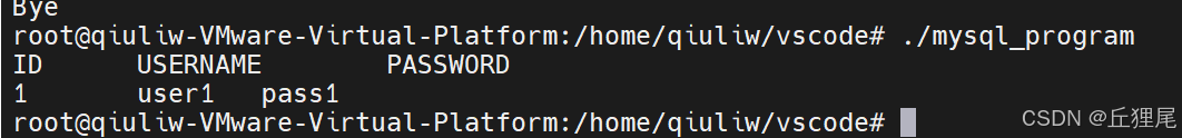
实验13 C语言连接和操作MySQL数据库
一、安装MySQL 1、使用包管理器安装MySQL sudo apt update sudo apt install mysql-server2、启动MySQL服务: sudo systemctl start mysql3、检查MySQL服务状态: sudo systemctl status mysql二、安装MySQL开发库 sudo apt-get install libmysqlcli…...
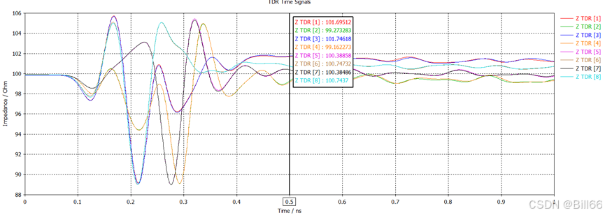
90度Floating B to B 高速连接器信号完整性仿真
在180度 B to B Connector 信号完整性仿真时,不会碰到端口设置不方便问题,但在做90度B to B Connector信号完整性仿真时就会碰到端口设置问题。如下面的90度B to B Connector。 公座 母座 公母对插后如下: 客户要求改Connector需符合PCI-E3.…...
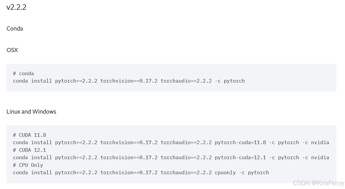
【踩坑】Pytorch与CUDA版本的关系及安装
Pytorch、CUDA和CUDA Toolkit区分 查看当前环境常用shell命令python脚本 Driver API CUDA(nvidia-smi)Runtime API CUDA(nvcc --version)pytorch选择CUDA版本的顺序安装需要的CUDA,多版本共存和自由切换 本文参考 http…...

信息隐藏 数字图像空域隐写与分析技术的实现
数字图像隐写与分析 摘要 随着信息技术的发展,隐写术作为一种信息隐藏技术,越来越受到关注。本文介绍了一种基于最低有效位(LSB)方法的数字图像隐写技术,并实现了隐写数据的嵌入与提取。通过卡方检验分析隐写图像的统计特性,评估隐写数据对图像的影响。实验结果表明,该…...

halcon单相机+机器人*眼在手外标定心得
目的 得到相机坐标系下的点与机器人底座base的转换关系,camera_in_base 两个不确定的定量 1,相机与机器人底座base之间的相对位置是固定的,既camera_in_base 2,机械手末端与标定物 tool_in_obj是固定的 辅助确定量 工作台与相…...

pytest入门十:配置文件
pytest.ini:pytest的主配置文件,可以改变pytest的默认行为conftest.py:测试用例的一些fixture配置 pytest.ini marks mark 打标的执行 pytest.mark.add add需要些marks配置否则报warning [pytest] markersadd:测试打标 测试用例中添加了 p…...
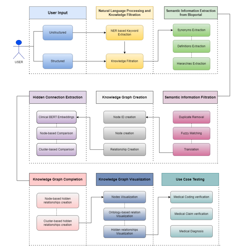
基于Clinical BERT的医疗知识图谱自动化构建方法,双层对比框架
基于Clinical BERT的医疗知识图谱自动化构建方法,双层对比框架 论文大纲理解1. 确认目标2. 目标-手段分析3. 实现步骤4. 金手指分析 全流程核心模式核心模式提取压缩后的系统描述核心创新点 数据分析第一步:数据收集第二步:规律挖掘第三步&am…...

介绍 Html 和 Html 5 的关系与区别
HTML(HyperText Markup Language)是构建网页的标准标记语言,而 HTML5 是 HTML 的最新版本,包含了一些新的功能、元素、API 和属性。HTML5 相对于早期版本的 HTML(比如 HTML4)有许多重要的改进和变化。以下是…...

C05S13-MySQL数据库备份与恢复
一、MySQL数据备份 1. 数据备份概述 数据备份的主要目的是灾难恢复,也就是当数据库等出现故障导致数据丢失,能够通过备份恢复数据。 数据备份可以分为物理备份和逻辑备份。物理备份,又称为冷备份,需要关闭数据库进行备份&#…...

【MySQL — 数据库基础】深入理解数据库服务与数据库关系、MySQL连接创建、客户端工具及架构解析
目录 1. 数据库服务&数据库&表之间的关系 1.1 复习 my.ini 1.2 MYSQL服务基于mysqld启动而启动 1.3 数据库服务的具体含义 1.4 数据库服务&数据库&表之间的关系 2. 客户端工具 2.1 客户端连接MySQL服务器 2.2 客…...
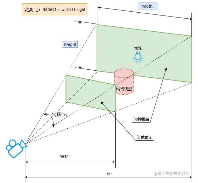
Three.js相机Camera控件知识梳理
原文:https://juejin.cn/post/7231089453695238204?searchId20241217193043D32C9115C2057FE3AD64 1. 相机类型 Three.js 主要提供了两种类型的相机:正交相机(OrthographicCamera)和透视相机(PerspectiveCamera&…...

Unity 开发Apple Vision Pro空间锚点应用Spatial Anchor
空间锚点具有多方面的作用 虚拟物体定位与固定: 位置保持:可以把虚拟物体固定在现实世界中的特定区域或位置。即使使用者退出程序后再次打开,之前锚定过的虚拟物体仍然能够出现在之前所锚定的位置,为用户提供连贯的体验。比如在一…...
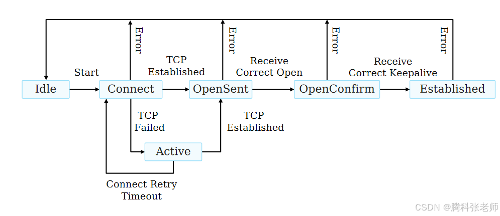
BGP的六种状态分别是什么?
此文章主要简单介绍下BGP的六种状态 1.Idle BGP会话的初始状态,路由器在此状态下不与任何BGP邻居通信,通常标识会话还没有开始或由于错误而未能启动,一般来说,缺乏去往BGP对等体的路由是导致BGP路由器其状态一直处于idle状态的常…...
IDEA搭建SpringBoot,MyBatis,Mysql工程项目
目录 一、前言 二、项目结构 三、初始化项目 四、SpringBoot项目集成Mybatis编写接口 五、代码仓库 一、前言 构建一个基于Spring Boot框架的现代化Web应用程序,以满足[公司/组织名称]对于[业务需求描述]的需求。通过利用Spring Boot简化企业级应用开发的优势&…...

Reactor
文章目录 正确的理解发送double free问题 1.把我们的reactor进行拆分2.链接管理3.Reactor的理论 listensock只需要设置_recv_cb,而其他sock,读,写,异常 所以今天写nullptr其实就不太对,添加为空就没办法去响应事件 获…...

在ESP32使用AT指令集与服务器进行TCP/IP通信时,<link ID> 解释
在ESP32使用AT指令集与服务器进行TCP/IP通信时,<link ID> 是一个非常重要的参数。它用于标识不同的连接实例,特别是在多连接场景下(如同时建立多个TCP或UDP连接)。每个连接都有唯一的<link ID>,通过这个ID…...

VMware 虚拟机 Kali Linux 光标消失?五步实操攻略轻松找回
在 VMware Workstation Pro 中运行 Kali Linux 时,不少用户会遇到 “光标隐形” 的棘手问题 —— 系统可正常操作,但光标一进入虚拟机窗口就消失。这一现象多由硬件兼容性、驱动配置或增强工具缺失导致,并非硬件故障。本文整合社区实测有效方…...
运动服爆炸图细节展示)
Nano-Banana Studio惊艳效果:高分辨率(1024x1024)运动服爆炸图细节展示
Nano-Banana Studio惊艳效果:高分辨率(1024x1024)运动服爆炸图细节展示 1. 开篇:当AI遇见设计拆解 你有没有遇到过这样的情况:想要展示一件运动服的所有设计细节,却不知道从哪里开始?传统的产…...

AMD显卡AI部署实战指南:ROCm模型运行与性能优化
AMD显卡AI部署实战指南:ROCm模型运行与性能优化 【免费下载链接】ollama-for-amd Get up and running with Llama 3, Mistral, Gemma, and other large language models.by adding more amd gpu support. 项目地址: https://gitcode.com/gh_mirrors/ol/ollama-for…...

记录一次 反射引起的Metaspace OOM 的完整排查
一、问题背景线上某个 Spring Boot 服务偶发出现:java.lang.OutOfMemoryError: MetaspaceJVM 参数中已经限制:-XX:MetaspaceSize512m -XX:MaxMetaspaceSize512m但监控显示:Metaspace used ≈ 370MB Metaspace committed ≈ 508MB看起来仍…...

PHP-JWT:PHP 中 JSON Web Tokens 的完整实现指南
PHP-JWT:PHP 中 JSON Web Tokens 的完整实现指南 【免费下载链接】php-jwt 项目地址: https://gitcode.com/gh_mirrors/ph/php-jwt Firebase PHP-JWT 是一个遵循 RFC 7519 标准的 PHP JSON Web Tokens 实现库,提供安全、高效的 JWT 编码和解码功…...

eSearch一站式屏幕效率工具安装指南
eSearch一站式屏幕效率工具安装指南 【免费下载链接】eSearch 截屏 离线OCR 搜索翻译 以图搜图 贴图 录屏 万向滚动截屏 屏幕翻译 Screenshot Offline OCR Search Translate Search for picture Paste the picture on the screen Screen recorder Omnidirectional scrolling sc…...

PlotJuggler颜色映射终极指南:如何创建惊艳的数据可视化效果
PlotJuggler颜色映射终极指南:如何创建惊艳的数据可视化效果 【免费下载链接】PlotJuggler The Time Series Visualization Tool that you deserve. 项目地址: https://gitcode.com/gh_mirrors/pl/PlotJuggler PlotJuggler是一款功能强大的时间序列数据可视化…...

smart-mqtt v1.5.4发布,认证能力大升级
smart-mqtt v1.5.4正式发布,此次版本聚焦企业级连接认证能力升级,推出全新高级认证插件,在高性能底座上补齐企业级接入能力,还公布了获取方式与未来规划。版本核心亮点v1.5.4重点通过advanced-auth-plugin让连接认证更适配企业真实…...

如何用FanControl彻底告别电脑噪音?Windows风扇控制终极解决方案
如何用FanControl彻底告别电脑噪音?Windows风扇控制终极解决方案 【免费下载链接】FanControl.Releases This is the release repository for Fan Control, a highly customizable fan controlling software for Windows. 项目地址: https://gitcode.com/GitHub_T…...

终极指南:Google Maps Python客户端错误处理与异常类型完全解析
终极指南:Google Maps Python客户端错误处理与异常类型完全解析 【免费下载链接】google-maps-services-python Python client library for Google Maps API Web Services 项目地址: https://gitcode.com/gh_mirrors/go/google-maps-services-python 在Pytho…...