当前位置：首页 > news >正文

贝叶斯优化相关

news 文章来源：https://blog.csdn.net/hbkybkzw/article/details/145338659 2025/5/14 7:44:30

贝叶斯优化相关

python中有很多模块支持贝叶斯优化，如bayesian-optimization、hyperopt，比较好用的是hyperopt，下面是对hyperopt文章的翻译，原文地址如下

https://districtdatalabs.silvrback.com/parameter-tuning-with-hyperopt

abstract

This post will cover a few things needed to quickly implement a fast, principled method for machine learning model parameter tuning. There are two common methods of parameter tuning: grid search and random search. Each have their pros and cons. Grid search is slow but effective at searching the whole search space, while random search is fast, but could miss important points in the search space. Luckily, a third option exists: Bayesian optimization. In this post, we will focus on one implementation of Bayesian optimization, a Python module called hyperopt.

这篇文章将介绍快速实现机器学习模型参数调整的快速、有原则的方法所需的一些内容。常用的参数调优方法有两种：网格搜索和随机搜索。每个都有其优点和缺点。网格搜索很慢，但在搜索整个搜索空间时很有效，而随机搜索很快，但可能会错过搜索空间中的重要点。幸运的是，存在第三种选择：贝叶斯优化。在这篇文章中，我们将重点介绍贝叶斯优化的一种实现，即一个名为 hyperopt 的 Python 模块。
Using Bayesian optimization for parameter tuning allows us to obtain the best parameters for a given model, e.g., logistic regression. This also allows us to perform optimal model selection. Typically, a machine learning engineer or data scientist will perform some form of manual parameter tuning (grid search or random search) for a few models - like decision tree, support vector machine, and k nearest neighbors - then compare the accuracy scores and select the best one for use. This method has the possibility of comparing sub-optimal models. Maybe the data scientist found the optimal parameters for the decision tree, but missed the optimal parameters for SVM. This means their model comparison was flawed. K nearest neighbors may beat SVM every time if the SVM parameters are poorly tuned. Bayesian optimization allow the data scientist to find the best parameters for all models, and therefore compare the best models. This results in better model selection, because you are comparing the best k nearest neighbors to the best decision tree. Only in this way can you do model selection with high confidence, assured that the actual best model is selected and used.

使用贝叶斯优化进行参数调整可以让我们获得给定模型的最佳参数，例如逻辑回归。这也使我们能够执行最佳模型选择。通常，机器学习工程师或数据科学家会对一些模型（如决策树、支持向量机和 k 个最近邻）执行某种形式的手动参数调整（网格搜索或随机搜索），然后比较准确度得分并选择最好的使用。这种方法有可能比较次优模型。也许数据科学家找到了决策树的最佳参数，但错过了 SVM 的最佳参数。这意味着他们的模型比较存在缺陷。如果 SVM 参数调整不佳，K 最近邻可能每次都击败 SVM。贝叶斯优化允许数据科学家找到所有模型的最佳参数，从而比较最佳模型。这会导致更好的模型选择，因为您正在将最佳 k 最近邻与最佳决策树进行比较。只有这样，您才能高枕无忧地进行模型选择，确保选择和使用实际的最佳模型。
Topics covered are in this post are:
1. Objective functions
2. Search spaces
3. Storing evaluation trials
4. Visualization
5. Full example on a classic dataset: Iris
To use the code below, you must install hyperopt and pymongo.

这篇文章中涉及的主题是：
1. 目标函数
2. 搜索空间
3. 存储评估试验
4. 可视化
5. 经典数据集的完整示例：鸢尾花
要使用下面的代码，您必须安装 hyperopt 和 pymongo。

Objective Functions - A Motivating Example

目标函数——一个启发性的例子*
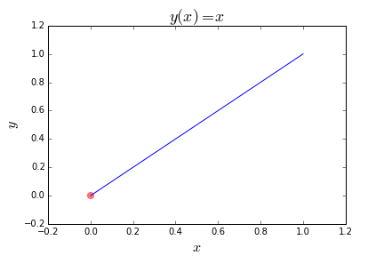
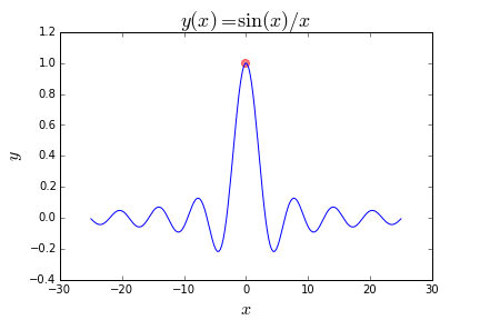
Suppose you have a function defined over some range, and you want to minimize it. That is, you want to find the input value that result in the lowest output value. The trivial example below finds the value of x that minimizes a linear function

假设您在某个范围内定义了一个函数，并且您希望最小化它。也就是说，您想要找到导致最低输出值的输入值。下面的简单示例找到使线性函数最小化的 x 值。
```
from hyperopt import fmin, tpe, hpbest = fmin(fn=lambda x: x   # fn接收一个最小化函数,space=hp.uniform('x' # 参数别名, 0 # 下限, 1 # 上限) # 指定搜索空间,algo=tpe.suggest # 采用搜索算法,max_evals=100 # 指定fmin函数将执行的最大评估次数)print(best)"""输出如下"""
{'x': 0.0002258846235372123}
```
Let’s break this down.

The function fmin first takes a function to minimize, denoted fn, which we here specify with an anonymous function lambda x: x. This function could be any valid value-returning function, such as mean absolute error in regression.

函数 fmin 首先采用一个最小化函数，记为 fn，我们在这里用匿名函数 lambda x: x 指定它。该函数可以是任何有效的值返回函数，例如回归中的平均绝对误差。

The next parameter specifies the search space, and in this example it is the continuous range of numbers between 0 and 1, specified by hp.uniform(‘x’, 0, 1). hp.uniform is a built-in hyperopt function that takes three parameters: the name, x, and the lower and upper bound of the range, 0 and 1.

下一个函数指定搜索空间，在此示例中他是由hp.uniform(‘x’,0,1)指定的0到1之间的连续数字范围。hp.uniform 是一个内置的 hyperopt 函数，它接受三个参数：名称 x 以及范围的下限和上限 0 和 1。

The parameter algo takes a search algorithm, in this case tpe which stands for tree of Parzen estimators. This topic is beyond the scope of this blog post, but the mathochistic reader may peruse this for details. The algo parameter can also be set to hyperopt.random, but we do not cover that here as it is widely known search strategy. However, in a future post, we can.

参数 algo 采用搜索算法，在本例中 tpe 代表 Parzen 估计器树。这个话题超出了这篇博文的范围，但是有数学背景的同学可以细读这篇文章。 algo 参数也可以设置为 hyperopt.random，但我们不在这里讨论它，因为它是众所周知的搜索策略。但是在未来的文章中我们可能会涉及。

Finally, we specify the maximum number of evaluations max_evals the fmin function will perform. This fmin function returns a python dictionary of values.An example of the output for the function above is {‘x’: 0.0002258846235372123}.

最后，我们指定 fmin 函数将执行的最大评估次数 max_evals。这个 fmin 函数返回一个 Python 值字典。上述函数的输出示例是{‘x’: 0.0002258846235372123}。

Here is the plot of the function. The red dot is the point we are trying to find.

这个是函数的图。红点是我们试图找到的点。

More Complicated Examples

一个更复杂的例子
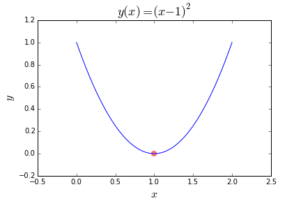
Here is a more complicated objective function: lambda x: (x-1)**2. This time we are trying to minimize a quadratic equation y(x) = (x-1)**2. So we alter the search space to include what we know to be the optimal value (x=1) plus some sub-optimal ranges on either side: hp.uniform('x', -2, 2).

Now we have:

这是一个更复杂的目标函数：lambda x: (x-1)**2。这次我们试图最小化一个二次方程 y(x) = (x-1)**2。所以我们改变搜索空间以包括我们知道的最优值 (x=1) 加上两边的一些次优范围：hp.uniform(‘x’, -2, 2)。

现在我们有：
```
from hyperopt import fmin,tpe,hpbest = fmin(fn=lambda x: (x-1)**2,space=hp.uniform('x', -2, 2),algo=tpe.suggest,max_evals=100)
print(best)
```
The output should look something like this:
```
"""输出如下"""
{'x': 0.9958194793700939}
```
Here is the plot.
Instead of minimizing an objective function, maybe we want to maximize it. To to this we need only return the negative of the function. For example, we could have a function y(x) = -(x**2):

有时候可能我们并不是想着最小化一个函数，而是最大化它。为此，我们只需要返回函数的负数即可。例如，我们可以有一个函数 y(x) = -(x**2)：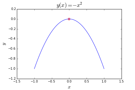

How could we go about solving this? We just take the objective function lambda x: -(x**2) and return the negative, giving lambda x: -1*-(x**2) or just lambda x: (x**2).

我们该如何解决这个问题？我们只取目标函数 lambda x: -(x2) 并返回负数，给出 lambda x: -1*-(x2) 或只是 lambda x: (x**2)。
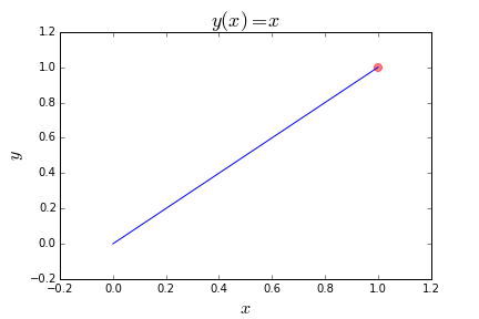
Here is one similar to example 1, but instead of minimizing, we are trying to maximize.

这是一个类似于示例 1 的示例，但我们不是最小化，而是试图最大化y=x。
Here is a function with many (infinitely many given an infinite range) local minima, which we are also trying to maximize:

这是一个具有许多（在无限范围内无限多）局部最小值的函数，我们也试图将其最大化：

Search Spaces

搜索空间
The hyperopt module includes a few handy functions to specify ranges for input parameters. We have already seen hp.uniform. Initially, these are stochastic search spaces, but as hyperopt learns more (as it gets more feedback from the objective function), it adapts and samples different parts of the initial search space that it thinks will give it the most meaningful feedback.

The following will be used in this post:
1. hp.choice(label, options) where options should be a python list or tuple.
2. hp.normal(label, mu, sigma) where mu and sigma are the mean and standard deviation, respectively.
3. hp.uniform(label, low, high) where low and high are the lower and upper bounds on the range.
hyperopt 模块包括一些方便的函数来指定输入参数的范围。我们已经看到了 hp.uniform。最初，这些是随机搜索空间，但随着 hyperopt 学习得更多（因为它从目标函数获得更多反馈），它会适应并采样它认为会给它最有意义的反馈的初始搜索空间的不同部分。

以下内容将在本文中使用：
1. hp.choice(label, options) 其中options应是 python 列表或元组。
2. hp.normal(label, mu, sigma) 其中mu和sigma分别是均值和标准差。
3. hp.uniform(label, low, high) 其中low和high是范围的下限和上限。
Others are available, such as hp.normal, hp.lognormal, hp.quniform, but we will not use them here.

To see some draws from the search space, we should import another function, and define the search space.

其他可用的相关函数，例如 hp.normal、hp.lognormal、hp.quniform，但我们不会在这里使用它们。

要查看搜索空间的一些绘制，我们应该导入另一个函数，并定义搜索空间。
```
import hyperopt.pyll.stochasticspace = {'x': hp.uniform('x', 0, 1),'y': hp.normal('y', 0, 1),'name': hp.choice('name', ['alice', 'bob']),
}print(hyperopt.pyll.stochastic.sample(space))
```
An example output is:
```
"""输出如下"""
{'name': 'alice', 'x': 0.7102704161240886, 'y': -1.102497756563188}
```

Capturing Info with Trials

通过Trials捕捉信息

It would be nice to see exactly what is happening inside the hyperopt black box. The Trials object allows us to do just that. We need only import a few more items.

如果能看到hyperopt黑匣子内发生了什么是极好的。Trials对象使我们能够做到这一点。我们只需要再导入一些东西。

from hyperopt import fmin, tpe, hp, STATUS_OK, Trialsfspace = {'x': hp.uniform('x', -5, 5)}def f(params):x = params['x']val = x**2return {'loss': val, 'status': STATUS_OK}trials = Trials()
best = fmin(fn=f, space=fspace, algo=tpe.suggest, max_evals=50, trials=trials)print('best:\n', best)print('trials:')
for trial in trials.trials[:2]:print(trial)

The STATUS_OK and Trials imports are new. The Trials object allows us to store info at each time step they are stored. We can then print them out and see what the evaluations of the function were for a given parameter at a given time step.

STATUS_OK和Trials是新导入的。Trials对象允许我们在每个时间步存储信息。然后我们可以将它们打印出来，并在给定的时间步查看给定参数的函数评估值。

Here is an example output of the code above:

"""输出如下"""
"""
需要注意的点
1. tid 是从0 到 max_evals-1
2. x(params)存储在misc中vals里
3. loss在result中（实际就是fmin函数返回的值）
"""best:{'x': -0.0008001691326020577}
trials:
{'state': 2, 'tid': 0, 'spec': None, 'result': {'loss': 0.08079044392675966, 'status': 'ok'}, 'misc': {'tid': 0, 'cmd': ('domain_attachment', 'FMinIter_Domain'), 'workdir': None, 'idxs': {'x': [0]}, 'vals': {'x': [-0.28423659849984073]}}, 'exp_key': None, 'owner': None, 'version': 0, 'book_time': datetime.datetime(2022, 4, 12, 14, 5, 15, 572000), 'refresh_time': datetime.datetime(2022, 4, 12, 14, 5, 15, 572000)
}{'state': 2, 'tid': 1, 'spec': None, 'result': {'loss': 15.862399717087962, 'status': 'ok'}, 'misc': {'tid': 1, 'cmd': ('domain_attachment', 'FMinIter_Domain'), 'workdir': None, 'idxs': {'x': [1]}, 'vals': {'x': [3.982762824609063]}}, 'exp_key': None, 'owner': None, 'version': 0, 'book_time': datetime.datetime(2022, 4, 12, 14, 5, 15, 573000), 'refresh_time': datetime.datetime(2022, 4, 12, 14, 5, 15, 573000)
}

The trials object stores data as a BSON object, which works just like a JSON object. BSON is from the pymongo module. We will not discuss the details here, but there are advanced options for hyperopt that require distributed computing using MongoDB, hence the pymongo import.

Back to the output above. The 'tid' is the time id, that is, the time step, which goes from 0 to max_evals-1. It increases by one each iteration. 'x' is in the 'vals' key, which is where your parameters are stored for each iteration. 'loss' is in the 'result' key, which gives us the value for our objective function at that iteration.

Let’s look at this in another way.

Trials对象将数据存储为BSON对象，其工作方式与JSON对象相同。BSON来自pymongo模块。我们不会在这里讨论细节，但是 hyperopt 有一些高级选项需要使用 MongoDB 进行分布式计算，因此需要导入 pymongo 。

‘tid’ 是时间 id，即时间步长，从 0 到 max_evals-1。它随着迭代次数递增。'x'是键'vals'的值，其中存储的是每次迭代参数的值。'loss'是键'result'的值，其给出了该次迭代目标函数的值。
Let’s look at this in another way.、

Visualization

We’ll go over two types of visualizations here:
1. val vs. time
2. loss vs. val.
First, val vs. time. Below is the code and sample output for plotting the trials.trials data described above.

我们将在这里讨论两种类型的可视化：val vs. time，以及 loss vs. val。首先，val vs time。下面是用于绘制上述 trial.trials 数据的代码和示例输出(为了效果，max_evals自己调到了5000)。
```
from hyperopt import fmin, tpe, hp, STATUS_OK, Trials
from matplotlib import pyplot as plt fspace = {'x': hp.uniform('x', -5, 5)}def f(params):x = params['x']val = x**2return {'loss': val, 'status': STATUS_OK}trials = Trials()
best = fmin(fn=f, space=fspace, algo=tpe.suggest, max_evals=5000, trials=trials)f, ax = plt.subplots(1)
xs = [t['tid'] for t in trials.trials] # tid 是从0 到 max_evals - 1
ys = [t['misc']['vals']['x'] for t in trials.trials] # 存储的是x（params）
ax.set_xlim(xs[0]-10, xs[-1]+10) 
ax.scatter(xs, ys, s=20, linewidth=0.01, alpha=0.75)
ax.set_title('$x$ $vs$ $t$ ', fontsize=18)
ax.set_xlabel('$t$', fontsize=16)
ax.set_ylabel('$x$', fontsize=16)
plt.show()
```
We can see that initially the algorithm picks values from the whole range equally (uniformly), but as time goes on and more is learned about the parameter’s effect on the objective function, the algorithm focuses more and more on areas in which it thinks it will gain the most - the range close to zero. It still explores the whole solution space, but less frequently.

Now let’s look at the plot of loss vs. val.

我们可以看到，最初算法从整个范围中均匀地选择值，但随着时间的推移以及参数对目标函数的影响了解越来越多，该算法越来越聚焦于它认为会取得最大收益的区域-一个接近零的范围。它仍然探索整个解空间，但频率有所下降。

现在让我们看看loss vs. val的图。
```
from hyperopt import fmin, tpe, hp, STATUS_OK, Trials
from matplotlib import pyplot as plt fspace = {'x': hp.uniform('x', -5, 5)}def f(params):x = params['x']val = x**2return {'loss': val, 'status': STATUS_OK}trials = Trials()
best = fmin(fn=f, space=fspace, algo=tpe.suggest, max_evals=5000, trials=trials)f, ax = plt.subplots(1)
xs = [t['misc']['vals']['x'] for t in trials.trials]
ys = [t['result']['loss'] for t in trials.trials]
ax.scatter(xs, ys, s=20, linewidth=0.01, alpha=0.75)
ax.set_title('$val$ $vs$ $x$ ', fontsize=18)
ax.set_xlabel('$x$', fontsize=16)
ax.set_ylabel('$val$', fontsize=16)
plt.show()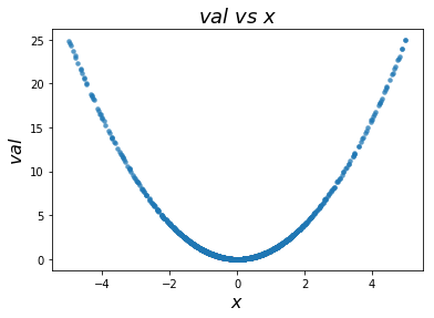
```
This gives us what we expect, since the function y(x) = x**2 is deterministic.

To wrap up, let’s try a more complicated example, with more randomness and more parameters.

这给了我们预期的结果，因为函数 y(x) = x**2 是确定性的。

最后，让我们尝试一个更复杂的例子，它有更多的随机性和更多的参数。

The Iris Dataset

In this section, we’ll walk through 4 full examples of using hyperopt for parameter tuning on a classic dataset, Iris. We will cover K-Nearest Neighbors (KNN), Support Vector Machines (SVM), Decision Trees, and Random Forests. Note that since we are trying to maximize the cross-validation accuracy (acc in the code below), we must negate this value for hyperopt, since hyperopt only knows how to minimize a function. Minimizing a function f is the same as maximizing the negative of f.

For this task, we’ll use the classic Iris data set, and do some supervised machine learning. There are 4 input features, and three output classes. The data are labeled as belonging to class 0, 1, or 2, which map to different kinds of Iris flower. The input has 4 columns: sepal length, sepal width, petal length, and pedal width. Units of the input are centimeters. We will use these 4 features to learn a model that predicts one of three output classes. Since the data is provided by sklearn, it has a nice DESCR attribute that provides details on the data set. Try the following for more details.

在本节中，我们将介绍 4 个使用 hyperopt 对经典数据集 Iris 进行参数调整的完整示例。我们将介绍 K 近邻 (KNN)、支持向量机 (SVM)、决策树和随机森林。请注意，由于我们试图最大化交叉验证的准确性（acc 在下面的代码中），我们必须对 hyperopt 取反，因为 hyperopt 只知道如何最小化函数。最小化函数 f 与最大化 f 的负值相同。

对于这个任务，我们将使用经典的 Iris 数据集，并进行一些监督机器学习。有 4 个输入特征和三个输出类。数据被标记为属于 0、1 或 2 类，它们映射到不同种类的鸢尾花。输入有 4 列：萼片长度、萼片宽度、花瓣长度和踏板宽度。输入的单位是厘米。我们将使用这 4 个特征来学习预测三个输出类别之一的模型。由于数据是由 sklearn 提供的，它有一个很好的 DESCR 属性，可以提供数据集的详细信息。请尝试以下操作以获取更多详细信息。
```
from sklearn.datasets import load_irisiris = load_iris()
print(iris.feature_names) # input names
print(iris.target_names) # output names
print(iris.DESCR) # everything else
```
Let’s get to know the data a little better through visualization of the features and classes, using the code below. Don’t forget to pip install seaborn if you have not already.

让我们通过使用下面的代码可视化特征和类来更好地了解数据。如果你还没安装别忘了先执行pip install searborn。
```
import seaborn as sns
import pandas as pdsns.set(style="whitegrid", palette="husl")iris = sns.load_dataset("iris")
print(iris.head())iris = pd.melt(iris, "species", var_name="measurement")
print(iris.head())f, ax = plt.subplots(1, figsize=(15,10))
sns.stripplot(x="measurement", y="value", hue="species", data=iris, jitter=True, edgecolor="white", ax=ax)
```
Here is the plot:

K-Nearest Neighbors

We now apply hyperopt to finding the best parameters to a K-Nearest Neighbor (KNN) machine learning model. The KNN model classifies a data point from the test set based on majority class of the k nearest data points in the training data set. More information on this algorithm can he found here.
The code below incorporates everything we have covered.

我们现在将使用hyperopt来找到 K近邻（KNN）机器学习模型的最佳参数。KNN 模型是基于训练数据集中 k 个最近数据点的大多数类别对来自测试集的数据点进行分类。关于这个算法的更多信息可以参考这里。下面的代码结合了我们所涵盖的一切。

from sklearn import datasets
from sklearn.model_selection import cross_val_score
from sklearn.neighbors import KNeighborsClassifieriris = datasets.load_iris()X = iris.data
y = iris.targetspace4knn = {'n_neighbors': hp.choice('n_neighbors', range(1,100))
}def f(params):clf = KNeighborsClassifier(**params)acc = cross_val_score(clf, X, y).mean()return {'loss': -acc, 'status': STATUS_OK}trials = Trials()best = fmin(f, space4knn, algo=tpe.suggest, max_evals=100, trials=trials)print('best:\n',best)"""输出如下"""
best:{'n_neighbors': 9}

Now let’s see the plot of the output. The y axis is the cross validation score, and the x axis is the k value in k-nearest-neighbors. Here is the code and its image:

现在让我们看看输出图。 y 轴是交叉验证分数，x 轴是knn中的 k 值。以下是代码及其图像：

f, ax = plt.subplots(1)#, figsize=(10,10))
xs = [t['misc']['vals']['n_neighbors'] for t in trials.trials]
ys = [-t['result']['loss'] for t in trials.trials]
ax.scatter(xs, ys, s=20, linewidth=0.01, alpha=0.5)
ax.set_title('Iris Dataset - KNN', fontsize=18)
ax.set_xlabel('n_neighbors', fontsize=12)
ax.set_ylabel('cross validation accuracy', fontsize=12)

外链图片转存失败,源站可能有防盗链机制,建议将图片保存下来直接上传

After k is greater than 69, the accuracy drops precipitously. This is due to the number of each class in the dataset. There are only 50 instances of each of the three classes. So let’s drill down by limiting the values of 'n_neighbors' to smaller values.

k大于63后，准确率急剧下降。这是由于数据集中每个类的数量。这三个类中的每一个只有 50 个实例。因此，让我们通过将“n_neighbors”的值限制为更小的值来深入研究。

from sklearn import datasets
from sklearn.model_selection import cross_val_score
from sklearn.neighbors import KNeighborsClassifieriris = datasets.load_iris()X = iris.data
y = iris.targetspace4knn = {'n_neighbors': hp.choice('n_neighbors', range(1,50))
}def f(params):clf = KNeighborsClassifier(**params)acc = cross_val_score(clf, X, y).mean()return {'loss': -acc, 'status': STATUS_OK}trials = Trials()best = fmin(f, space4knn, algo=tpe.suggest, max_evals=100, trials=trials)print('best:\n',best)f, ax = plt.subplots(1)#, figsize=(10,10))
xs = [t['misc']['vals']['n_neighbors'] for t in trials.trials]
ys = [-t['result']['loss'] for t in trials.trials]
ax.scatter(xs, ys, s=20, linewidth=0.01, alpha=0.5)
ax.set_title('Iris Dataset - KNN', fontsize=18)
ax.set_xlabel('n_neighbors', fontsize=12)
ax.set_ylabel('cross validation accuracy', fontsize=12)"""输出如下"""
{'n_neighbors': 5}

Here is what we get when we run the same code for visualization:

外链图片转存失败,源站可能有防盗链机制,建议将图片保存下来直接上传

Now we can see clearly that there is a best value for k, at k = 5

The model above does not do any preprocessing. So let’s normalize and scale our features and see if that helps. Use this code:

现在我们可以清楚地看到 k 有一个最佳值，在 k = 4。

上面的模型不做任何预处理。所以让我们使用以下代码规范化和扩展我们的特征，看看是否有帮助。

# now with scaling as an option
from sklearn import datasets
from sklearn.model_selection import cross_val_score
from sklearn.neighbors import KNeighborsClassifier
from sklearn.preprocessing import StandardScaler
from sklearn.preprocessing import MinMaxScaler
import numpy as npiris = datasets.load_iris()
X = iris.data
y = iris.targetspace4knn = {'n_neighbors': hp.choice('n_neighbors', range(1,50)),'scale': hp.choice('scale', [0, 1]),'normalize': hp.choice('normalize', [0, 1])
}def f(params):X_ = X[:]if 'normalize' in params:if params['normalize'] == 1:normalize = MinMaxScaler()X_ = normalize.fit_transform(X_)del params['normalize']if 'scale' in params:if params['scale'] == 1:scale = StandardScaler()X_ = scale.fit_transform(X_)del params['scale']clf = KNeighborsClassifier(**params)acc = cross_val_score(clf, X_, y).mean()    return {'loss': -acc, 'status': STATUS_OK}trials = Trials()
best = fmin(f, space=space4knn, algo=tpe.suggest, max_evals=100, trials=trials)print('best:\n',best)"""输出如下"""
{'n_neighbors': 5, 'normalize': 0, 'scale': 0}

And plot the parameters like this:

parameters = ['n_neighbors', 'scale', 'normalize']
cols = len(parameters)
f, axes = plt.subplots(nrows=1, ncols=cols, figsize=(15,5))
cmap = plt.cm.jet
for i, val in enumerate(parameters):xs = np.array([t['misc']['vals'][val] for t in trials.trials]).ravel()ys = [-t['result']['loss'] for t in trials.trials]xs, ys = zip(*sorted(zip(xs, ys)))ys = np.array(ys)axes[i].scatter(xs, ys, s=20, linewidth=0.01, alpha=0.75, c=cmap(float(i)/len(parameters)))axes[i].set_title(val)

外链图片转存失败,源站可能有防盗链机制,建议将图片保存下来直接上传

We see that scaling and/or normalizing the data does not improve predictive accuracy. The best value of k remains 5, which results in 98.6 % accuracy.

So this is great for parameter tuning a simple model, KNN. Let’s see what we can do with Support Vector Machines (SVM).

我们看到缩放和/或规范化数据并不能提高预测准确性。 k 的最佳值仍然是 5，这导致 98.6% 的准确度。

所以，这对于调整简单模型 KNN 的参数非常有用。让我们看看我们可以用支持向量机 (SVM) 做什么。

Support Vector Machines (SVM)

Since this is a classification task, we’ll use sklearn’s SVC class. Here is the code:

由于这是一个分类任务，我们将使用 sklearn 的 SVC 类。

from sklearn import datasets
from sklearn.model_selection import cross_val_score
from sklearn.neighbors import KNeighborsClassifier
from sklearn.svm import SVC
from sklearn.preprocessing import StandardScaler
from sklearn.preprocessing import MinMaxScaler
import numpy as npiris = datasets.load_iris()
X = iris.data
y = iris.targetspace4svm = {'C': hp.uniform('C', 0, 20),'kernel': hp.choice('kernel', ['linear', 'sigmoid', 'poly', 'rbf']),'gamma': hp.uniform('gamma', 0, 20),'scale': hp.choice('scale', [0, 1]),'normalize': hp.choice('normalize', [0, 1])
}def f(params):X_ = X[:]if 'normalize' in params:if params['normalize'] == 1:normalize = MinMaxScaler()X_ = normalize.fit_transform(X_)del params['normalize']if 'scale' in params:if params['scale'] == 1:scale = StandardScaler()X_ = scale.fit_transform(X_)del params['scale']clf = SVC(**params)acc = cross_val_score(clf, X_, y).mean()    return {'loss': -acc, 'status': STATUS_OK}trials = Trials()
best = fmin(f, space4svm, algo=tpe.suggest, max_evals=100, trials=trials)
print('best:\n',best)parameters = ['C', 'kernel', 'gamma', 'scale', 'normalize']
cols = len(parameters)
f, axes = plt.subplots(nrows=1, ncols=cols, figsize=(20,5))
cmap = plt.cm.jet
for i, val in enumerate(parameters):xs = np.array([t['misc']['vals'][val] for t in trials.trials]).ravel()ys = [-t['result']['loss'] for t in trials.trials]xs, ys = zip(*sorted(zip(xs, ys)))axes[i].scatter(xs, ys, s=20, linewidth=0.01, alpha=0.25, c=cmap(float(i)/len(parameters)))axes[i].set_title(val)axes[i].set_ylim([0.9, 1.0])"""输出如下"""{'C': 0.7168209011868267, 'gamma': 3.7409805767298074, 'kernel': 0, 'normalize': 0, 'scale': 0}

Here is what we get: 外链图片转存失败,源站可能有防盗链机制,建议将图片保存下来直接上传

Again, scaling and normalizing do not help. The first choice of kernel funcion is the best (linear), the best C value is 0.7168209011868267, and the best gamma is 3.7409805767298074. This set of parameters results in 99.3 % classification accuracy.

Decision Trees

We will only attempt to optimize on a few parameters of decision trees. Here is the code.

我们只会尝试优化决策树的几个参数。

from sklearn import datasets
from sklearn.model_selection import cross_val_score
from sklearn.neighbors import KNeighborsClassifier
from sklearn.tree import DecisionTreeClassifier
from sklearn.svm import SVC
from sklearn.preprocessing import StandardScaler
from sklearn.preprocessing import MinMaxScaler
import numpy as npiris = datasets.load_iris()
X_original = iris.data
y_original = iris.targetspace4dt = {'max_depth': hp.choice('max_depth', range(1,20)),'max_features': hp.choice('max_features', range(1,5)),'criterion': hp.choice('criterion', ["gini", "entropy"]),'scale': hp.choice('scale', [0, 1]),'normalize': hp.choice('normalize', [0, 1])
}def f(params):X_ = X[:]if 'normalize' in params:if params['normalize'] == 1:normalize = MinMaxScaler()X_ = normalize.fit_transform(X_)del params['normalize']if 'scale' in params:if params['scale'] == 1:scale = StandardScaler()X_ = scale.fit_transform(X_)del params['scale']clf = DecisionTreeClassifier(**params)acc = cross_val_score(clf, X_, y).mean()    return {'loss': -acc, 'status': STATUS_OK}trials = Trials()
best = fmin(f, space4dt, algo=tpe.suggest, max_evals=300, trials=trials)
print('best:',best)

The output is the following, which gives 97.3 % accuracy.

"""输出如下"""
best: {'criterion': 0, 'max_depth': 6, 'max_features': 2, 'normalize': 0, 'scale': 0}

Here are the plots. We can see that there is little difference in performance with different values of scale, normalize, and criterion.

我们可以看到，在 scale、normalize 和 criterion 的不同值下，性能差异不大。

parameters = ['max_depth', 'max_features', 'criterion', 'scale', 'normalize'] # decision tree
cols = len(parameters)
f, axes = plt.subplots(nrows=1, ncols=cols, figsize=(20,5))
cmap = plt.cm.jet
for i, val in enumerate(parameters):xs = np.array([t['misc']['vals'][val] for t in trials.trials]).ravel()ys = [-t['result']['loss'] for t in trials.trials]xs, ys = zip(*sorted(zip(xs, ys)))ys = np.array(ys)axes[i].scatter(xs, ys, s=20, linewidth=0.01, alpha=0.5, c=cmap(float(i)/len(parameters)))axes[i].set_title(val)#axes[i].set_ylim([0.9,1.0])

外链图片转存失败,源站可能有防盗链机制,建议将图片保存下来直接上传

Random Forests

Let’s see what’s happending with an ensemble classifier, Random Forest, which is just a collection of decision trees trained on different even-sized partitions of the data, each of which votes on an output class, with the majority class being chosen as the prediction.

让我们来看看集成分类器随机森林发生了什么，随机森林只是在不同分区数据上训练的决策树集合，每个分区都对输出类进行投票，并将绝大多数类的选择为预测

from sklearn import datasets
from sklearn.model_selection import cross_val_score
from sklearn.neighbors import KNeighborsClassifier
from sklearn.tree import DecisionTreeClassifier
from sklearn.ensemble import RandomForestClassifier
from sklearn.svm import SVC
from sklearn.preprocessing import StandardScaler
from sklearn.preprocessing import MinMaxScaler
import numpy as npiris = datasets.load_iris()
X = iris.data
y = iris.targetspace4rf = {'max_depth': hp.choice('max_depth', range(1,20)),'max_features': hp.choice('max_features', range(1,5)),'n_estimators': hp.choice('n_estimators', range(1,20)),'criterion': hp.choice('criterion', ["gini", "entropy"]),'scale': hp.choice('scale', [0, 1]),'normalize': hp.choice('normalize', [0, 1])
}best = 0def f(params):global bestX_ = X[:]if 'normalize' in params:if params['normalize'] == 1:normalize = MinMaxScaler()X_ = normalize.fit_transform(X_)del params['normalize']if 'scale' in params:if params['scale'] == 1:scale = StandardScaler()X_ = scale.fit_transform(X_)del params['scale']clf = RandomForestClassifier(**params)acc = cross_val_score(clf, X_, y).mean()    if acc > best:best = accprint('new best:', best, params)return {'loss': -acc, 'status': STATUS_OK}trials = Trials()
best = fmin(f, space4rf, algo=tpe.suggest, max_evals=300, trials=trials)
print('best:\n',best)"""输出如下"""
new best:                                                                                                              
0.9666666666666668                                                                                                     
{'criterion': 'gini', 'max_depth': 8, 'max_features': 4, 'n_estimators': 9
}        new best:                                                                                                              
0.9800000000000001                                                                                                     
{'criterion': 'gini', 'max_depth': 18, 'max_features': 3, 'n_estimators': 6
}    best:{'criterion': 0, 'max_depth': 17, 'max_features': 2, 'n_estimators': 5, 'normalize': 0, 'scale': 0}

Again, we only get 97.3 % accuracy, same as decision tree.

Here is the code to plot the parameters:

parameters = ['n_estimators', 'max_depth', 'max_features', 'criterion', 'scale', 'normalize']
f, axes = plt.subplots(nrows=2, ncols=3, figsize=(15,10))
cmap = plt.cm.jet
for i, val in enumerate(parameters):print(i, val)xs = np.array([t['misc']['vals'][val] for t in trials.trials]).ravel()ys = [-t['result']['loss'] for t in trials.trials]xs, ys = zip(*sorted(zip(xs, ys)))ys = np.array(ys)axes[i//3,i%3].scatter(xs, ys, s=20, linewidth=0.01, alpha=0.5, c=cmap(float(i)/len(parameters)))axes[i//3,i%3].set_title(val)#axes[i/3,i%3].set_ylim([0.9,1.0])"""输出如下"""
0 n_estimators
1 max_depth
2 max_features
3 criterion
4 scale
5 normalize

外链图片转存失败,源站可能有防盗链机制,建议将图片保存下来直接上传

All Together Now

While it is fun and instructive to automatically tune the parameters of one model - SVM or KNN, for example - it is more useful to tune them all at once and arrive at a best model overall. This allows us to compare all parameters and all models at once, which gives us the best model. Here is the code.

自动调整一个模型的参数（如SVM或KNN）非常有趣并且具有启发性，但同时调整它们并取得全局最佳模型则更有用。这使我们能够一次比较所有参数和所有模型，因此为我们提供了最佳模型。代码如下：

from sklearn import datasets
from sklearn.model_selection import cross_val_score
from sklearn.neighbors import KNeighborsClassifier
from sklearn.tree import DecisionTreeClassifier
from sklearn.naive_bayes import BernoulliNB
from sklearn.ensemble import RandomForestClassifier
from sklearn.svm import SVC
from sklearn.preprocessing import StandardScaler
from sklearn.preprocessing import MinMaxScaler
import numpy as npdigits = datasets.load_digits()
X = digits.data
y = digits.target
print(X.shape, y.shape)def hyperopt_train_test(params):t = params['type']del params['type']if t == 'naive_bayes':clf = BernoulliNB(**params)elif t == 'svm':clf = SVC(**params)elif t == 'dtree':clf = DecisionTreeClassifier(**params)elif t == 'knn':clf = KNeighborsClassifier(**params)else:return 0return cross_val_score(clf, X, y).mean()space = hp.choice('classifier_type', [{'type': 'naive_bayes','alpha': hp.uniform('alpha', 0.0, 2.0)},{'type': 'svm','C': hp.uniform('C', 0, 10.0),'kernel': hp.choice('kernel', ['linear', 'rbf']),'gamma': hp.uniform('gamma', 0, 20.0)},{'type': 'randomforest','max_depth': hp.choice('max_depth', range(1,20)),'max_features': hp.choice('max_features', range(1,5)),'n_estimators': hp.choice('n_estimators', range(1,20)),'criterion': hp.choice('criterion', ["gini", "entropy"]),'scale': hp.choice('scale', [0, 1]),'normalize': hp.choice('normalize', [0, 1])},{'type': 'knn','n_neighbors': hp.choice('knn_n_neighbors', range(1,50))}
])count = 0
best = 0
def f(params):global best, countcount += 1acc = hyperopt_train_test(params.copy())if acc > best:print('new best:', acc, 'using', params['type'])best = accif count % 50 == 0:print('iters:', count, ', acc:', acc, 'using', params)return {'loss': -acc, 'status': STATUS_OK}trials = Trials()
best = fmin(f, space, algo=tpe.suggest, max_evals=1500, trials=trials)
print('best:\n','best:')

This code takes a while to run since we increased the number of evaluations: max_evals=1500. There is also added output to update you when a new best accuracy is found. Curious as to why using this method does not find the best model that we found above: SVM with kernel=linear, C=1.416, and gamma=15.042.

由于我们增加了评估数量，此代码需要一段时间才能运行完：max_evals=1500。当找到新的最佳准确率时，它还会添加到输出用于更新。好奇为什么使用这种方法没有找到前面的最佳模型：参数为kernel=linear，C=1.416，gamma=15.042的SVM。

Conclusion

We have covered simple examples, like minimizing a deterministic linear function, and complicated examples, like tuning random forest parameters. The documentation for hyperopt is here. Another good blog on hyperopt is this one by FastML. A SciPy Conference paper by the hyperopt authors is Hyperopt: A Python Library for Optimizing the Hyperparameters of Machine Learning Algorithms, with an accompanying video tutorial. A more techical treatment of the engineering ins and outs is Making a Science of Model Search.

我们已经介绍了简单的例子，如最小化确定的线性函数，以及复杂的例子，如调整随机森林参数。hyperopt的官方文档在这里。另一篇有关 hyperopt 不错的博客位于 FastML 站点（译注：已无效）。hyperopt作者的SciPy会议论文是Hyperopt: A Python Library for Optimizing the Hyperparameters of Machine Learning Algorithms，伴随一起的视频教程。关于工程来龙去脉的更多技术处理细节可以参见Making a Science of Model Search。

The techniques in this post can be used in many domains other than machine learning, such as tuning the epsilon parameter in an epsilon-greedy multi-armed bandit, or the parameters passed to a graph generator to make a synthetic network that has certain properties. We will write more on that later.

这篇文章中的技术可以用于机器学习以外的许多领域，例如调整 epsilon-greedy 多臂老虎机中的“epsilon”参数，或者将参数传递给图形生成器以制作具有一定特性。我们稍后会写更多。